Conics in the hyperbolic plane

Theses Digitization Project John M. Pfau Library

2007

Conics in the hyperbolic plane

Conics in the hyperbolic plane

Trent Phillip Naeve

Follow this and additional works at: https://scholarworks.lib.csusb.edu/etd-project

Part of the Geometry and Topology Commons

Recommended Citation Recommended Citation

Naeve, Trent Phillip, "Conics in the hyperbolic plane" (2007). Theses Digitization Project. 3075.

https://scholarworks.lib.csusb.edu/etd-project/3075

A Thesis

Presented to the

Faculty of

California State University,

San Bernardino

In Partial Fulfillment

of the Requirements for the Degree

Master of Arts

in

Mathematics

by

Trent Phillip Naeve

A Thesis

Presented to the

Faculty of

California State University,

San Bernardino

by

Trent Phillip Naeve

June 2007

Chetan Prakash, Committee Member

r/o T

-Date

Peter Williams, Chair, Department of Mathematics

Chavez

Abstract

Let us consider the locus of intersection L D T (L), as L runs through the entire

pencil of lines through a point P where T is an affine transformation such that T (P) = Q.

This locus is an affine conic and any affine conic can be produced from this incidence

construction. The affine type of the conic (ellipse, parabola, hyperbola) is determined by

the invariants of T, the determinant and trace of its linear part. The purpose of this thesis

is to obtain a corresponding classification in the hyperbolic plane of conics defined by this

construction. We will use the Poincare disk as our model of the hyperbolic plane, whereby

T is a linear fractional transformation that preserves the disk. So th at our classification

is not model-dependent we will show that the conic produced by T is mapped to an affine

conic when dilation about the center of the disk by a hyperbolic factor of 2 is imposed.

The resulting intersections of this affine conic with the boundary of the disk coincide with

those of the hyperbolic locus, and this hyperbolic conic can be recovered in explicit form

by contracting the affine conic. We will find th at the type of conic is determined not only

Acknowledgements

I would like to dedicate this project to my brother, Christopher Todd Naeve

(1968-2006). This loss was drastic and devastating, but I was able to perservere with

extreme focus and concentration. He was always proud of all of my accomplishments and

I know he will be proud of this one. Chris was more than ju st my brother, he was a

father, a great companion and a good friend. I love and miss him very much.

I would like to thank Dr. John Sarli, without him, none of this could be possible.

I appreciate the time and effort th at Dr. Sarli devoted to me, as well as, his vast knowledge

and expertise. My only regret is th at I had only one opportunity for him to be my

instructor during my course of study. The experience of working on my project with Dr.

Sarli was the highlight of my M aster’s program.

I would also like to thank all my friends and family th at have supported and

Table of Contents

A bstract iii

A cknow ledgem ents iv

List o f Figures vi

1 Introdu ction 1

2 T he Affine P lan e 3

3 H yperbolic P lan e 21

4 Spinor C orrespondence 29

5 C lassification o f H yperbolic Conics 36

6 C onclusion 54

List of Figures

2.1 The intersections of L and T (L) that create an ellipse... 2.2 The ellipse... 2.3 The intersections of L and T (L) that create the parabola... 2.4 The parabola... 2.5 The intersections of L and T (L) that create the hyperbola... 2.6 The hyperbola...

4.1 A hyperbola created by the opposite case. ... 4.2 The contracted conic...

5.1 The ellipse with no intersections... 5.2 The ellipse with a unigue intersection, a single tangent... 5.3 The ellipse with two intersections, both tangents... 5.4 The ellipse with two intersections, a secant... 5.5 The ellipse with two intersections, a tangent and a secant... 5.6 The ellipse with two intersections, two secants... 5.7 The ellipse with no intersections... 5.8 The ellipse with one unique intersection... 5.9 The ellipse with two intersections as tangents... 5.10 The ellipse with two intersections as a secant... 5.11 The ellipse with three intersections... 5.12 The ellipse with four intersections...

Chapter 1

Introduction

W hat is a conic? The name comes from the work of the Greek mathematicians

Apollonius and Menaechmus who studied the intersection of planes with cones and prop­

erties of the resulting ellipses, parabolas, and hyperbolas [BEG99]. We associate these

curves with second-degree polynomial equations, th at is every second degree equation

represents a conic. Most texts define conics in terms of a focus and a directrix. These

are im portant metric properties but do not give any indication of how conics arise syn­

thetically in geometry. The study of conics is well over 2,000 years old and has given rise

to some of the most beautiful and striking results in geometry.

Conics arise in a planar geometry as a linear correspondence between a pair of

pencils [Ped88]. We can classify and produce affine conics by using the following theorem

which we will prove

T heorem 1.1. I f P and Q are points of the affine plane a n d T is an affine transformation

such that T (P) = Q, then the locus of intersections L d T (P), as L runs through the

entire pencil of lines through P, is a conic.

We will show th at the equation of this conic is

ex2 + (d — a )x y — by2 — (a + d )r y — cr2 = 0

where T is represented by the matrix:

_ ( ax by r

(1 +

and P = (—r, 0) and Q = (r, 0).

In the affine plane, the invariants of T, the determinant 5 and the trace t of the matrix, will allow us to classify the conic. The goal is to find invariants of T in the

hyperbolic plane th at function as the trace and determinant in the affine plane.

Poincare’s conformal disk model will be used, where points are those of the open

unit disk and lines are circular arcs orthogonal to the unit circle.

Choosing two points P and Q in the hyperbolic plane, a transformation T such

that T (P) = Q is now a conformal hyperbolic transformation T takes the pencils of lines

(arcs) through P to the pencil through Q. As in the affine plane, the locus of intersections

will define a conic. In order to classify the conic determined by T we will use a property

of the Poincare model th at relates to the Lobachevsky chord model, specifically, dilation

about the center of the disk by a hyperbolic factor of two takes the arc th at represents the

line to the chord of the disk with the same boundary points. This dilation gives rise to a

map from the group of hyperbolic transformations into the Euclidean affine group. This

so-called “spinor” map then allows us to place the hyperbolic conic in the same category

as its affine counterpart.

The result of this work will show that, while in the affine plane a conic can be

classified by three types of cases: an ellipse, a parabola, and a hyperbola, in the hyper­

bolic plane, conics are classified as one of six types: no intersection, unique intersection,

two intersections with either both tangents or a secant, three intersections, and four in­

tersections. Each case is determined by the number of intersections the conic has with

Chapter 2

The Affine Plane

In geometry, affine transformations of the plane map lines to lines, parallel lines

to parallel lines, and preserve ratios of lengths along lines [BEG99]. The affine linear

transformation T will be defined by linear equations such that:,

X = ax + by + p

Y = ex + dy + q

for some constants a, b, c, d,p, q. The transformation T must also be invertible (det ad —

be 7^ 0) and will be written as a matrix equation,

a b p f x \ ax + by + p

T (z, y) = c d q _y = ex + dy + q

V 0 l ) V J

1 /

a b

c d

x

+ P

Q y

be—ad

be—ad

- l

- l

d —b

—c a

dp — bq

—cp + aq

so,

and

X

y =

\ i !

d —b dp—bq \

be—ad —cp+aq

be—ad

1 /

ad—be —c ad—be a ad—be 0 ad—be 0

d „ —b 1, dp—bq ad—be'1' ad—be " be—ad ~C T a ii —cp+aq a d - b c J' ad—b ed be—ad

The above is the general theory where

- l

is the linear part and is the

T 1(x,y)

c d

a b

c d

l

l

V

a b

c d x

y

P

Q a b

c d

P

Q

P

Q

translation part.

For a specific case we will select two points P and Q th at will make the distance

between them arbitrary. Let P = (—r, 0) and Q = (r, 0). So our transformation T is

T

' a b p ' ' X ’ ' X '

c d q _y = _y

O

o _{I i /} I i /

f —r \

0

\ 1 /

/ r \

0

\ 1 /

a b

c d

\ 0 0

P

Q

V

then solve for p and q

—ar + 6(0) + p = r

—cr + d (0) + q = 0

. p = r + ar and

q = cr p = r (1 + a)

since T (P) = Q. The line L through P (—r, 0) with slope m is represented by the following

equation:

y - y i = m ( x - x i )

y — 0 = m ( x + r)

y = m (x + r)

and the transformation T is represented by

a b r (1 + a)

T = c d

\ 0 0

cr

1 so

and

/ -4

T-i =

ad—be \ 0

d+ ad—bc ad—be be—ad

a — c

ad—be

0

be—ad

1

\

’ X _{a d -b c '^ ad—bcP be—ad} ■ r '

y _ ~ c -r a ti —c

ad—bcJ' a d -b c y be—ad

must satisfy line L through point P (—r, 0) with slope m:

y — m ( x + r ) .

This yields,

^ x +

+ ( a ■r)

ad-ad,^Tcx + ^ b - cy - bc—ad

m {^bix - ^=rcy +

•r + r)

m {-^b-cx - ^ y +

■r +r)

___ C_ ,___a________ cr

ad—be'1' ad—b e y be­ ad

n

xm - ^b-cym +

ad

=b~cy + ^b-cym

xm +

+

( P+bmA I a d -b c 1 y

f a s h

I dm + c \ i d m + a d m —bem + bem —a dm , „ , c

y a d —bcJ ’ be—ad ' ' be—ad

( d m + c \ , d m + c ,„

y ad— be J x ~r (,c_ o(/ '

_ I dm + c . a d -b c \ _ i f d m + c _ ad—be A „ \ ad—be a+ bm J x 1 be—ad a+ bm J '

( d r r + c ] _ f d m + c \ y a + b m J J' y a + b mJ

y =

which is the equation of T (£).

Finally, we must determine the intersection of L with T (L) as L runs through

the pencil of P and describe this locus of points of intersection.

If we solve for m in the equation for L,

L : y = m ( x

+ r)

T ( L ) :

(®—r)

c+d™ (T _ a+bm ' >

c+d(^+ )

“+6(4 ? )

x —r

-JL~ x —r

c ( s + r ) + d y

x + r a ( x + r ) + b y

x + r

J L -x —r

c (x + r)+ d y a (x+ r)+ b y

x —r

cx+ cr+ d y a x+ ar+ by

1 ' g+r

a 1 b y '

1 ' ®+r

y (ax + ar + by)

axy + ary + by2

= (x — r) (ex + cr + dy)

ex2 + arx + dxy — crx — cr2 — dry9

--- S W * 1

2 _

ex2 — axy + dxy — by2 — ary — dry — cr 0

ex2 + (d — a) x y — by2 — (a + d )r y — cr2 = 0.

This is the equation of the affine conic (ellipse, parabola, or hyperbola) created by the

locus of points of intersection [Sar03].

The affine conic is determined by the invariants of T , the determinant and trace

of its linear parts. The type of conic in the Cartesian plane is determined by the co­

efficients of quadratic terms, so the type of conic depends only on the coefficients of x ( a b \

and y in the definition of T. Recall that in the m atrix T = the determinant

A = c ^ ( d - a )

j (d - a) —b

= —cb — 5 (d — a)2

-- —cb — | (d2 — 2ad + a2)

= (ad — cb) — | (d2 + 2ad + a2)

= (ad — cb) — | (a + d)2

will be an ellipse if A > 0, a parabola if A = 0, or a hyperbola if A < 0. Now we can

distinguish the type of conic strictly in terms of the determinant 8 and trace t and are able to summarize the results into the following theorem:

T heorem 2.1. The conic determined by P ,Q and transformation T is an ellipse if

r 2 < 48, a parabola if t2 = 4d , or a hyperbola if t2 > 48.

Let’s consider the following three cases: 1) ellipse, 2) parabola, and 3) hyper­

bola, where point P (—1,0) —> Q (1,0) and a, b, c, d are chosen at random and create the

equation of each conic:

Case 1: The Ellipse

Let a = —3, b = —2, c = 3, d = —2 and r = 1,

p = r (1 + a) q — rc

so = l (l + (-3 )) and = (1) (3)

= —2 = 3

( - 3 - 3 —2 \

and the matrix T = 3 —2 3

V 0 0 1 )

We will use the determinant d and trace t of the m atrix to verify th at the conic is an

ellipse,

= ad — be

= (-3 ) (-2 ) - (3) (-2 )

= 6 + 6

= 12

& d T2 < 48

(-3 ) + (-2 ) ( - 5 ) 2 < 4(12)

- 5 25 < 48

so the conic is an ellipse.

The m atrix of is

so T- l

and T - 1

( x \

y

\ 1 y

=2. 2.

12 12

= 3

12 12

= 5 \ 6 1 6 ^ 1 4

v o o i y v i y

z

Z

- 1 -X 1

y T X - p y ₄

V

J

I

7

must satisfy L through P (—1,0) with y = m (x + 1) so T (Z):

y = m(a: + l)

+ ? = r n ( - ± x + l y -

j + l)

= - ^ m x + ^m y + ^m

■ \ y - l m y

/ 1 \

0

z - i \

0

-|m+ _£4I _ I ° - V - r _L_ __ 6- ■

I I ™ * + Z l_ I

— 2 m + 3

a t — ____1?__ /p _1_ 12 .

y — —3 ~ 2 m 'b ' - 3 - 2i

- 2 m + 3 ™ i 2 m —3

.a - - r

—3 —2 m " —3—2m

T ( £ ) : y = —2 m + 3 ( —2 m —3 _ -I \L > •

Solve line L for m, (m = and substitute in T (L) to find the equation of the conic:

T ^ - - y =

_2Z_ 2—1

x —1

2y2 - 3xy - 3y

~ 2 y2 - 3xy - 3y

3x2 + x y + 2y2 + 5y - 3

^^■—3_{x+l °}

_ - 2 y + 3 a:+ 3

—2y—3a;—3

= (x - 1) (—2y + 3x + 3)

= —2xy + 3a:2 + 3a: + 2y — 3a: — 3

= 0

is the equation of the ellipse.

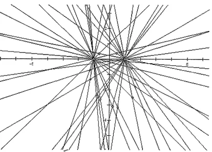
Graphing the conic gives a visual of the locus of intersection. First, choose

Ln : y = ra (a; + 1) - > T ( L n) : _{y =} —2 m + 3 / —2 m —3

i x : y = x + 1 - > T ( L i) : _{y =} ^ + 1

L 2 : _y = 2x + 2 - > T { L 2y. _{y = 4X} _ l7

L 3 : y — 3x + 3 - > T { L 3y . _{y = 3 X} _ 1₃

l4 - y = —x — 1 - > T { L 4)-. _{y = —5x} + 5

L 5 : _{y = —2x —} 2 -4- T ( L 5): _{y = - 7 s - 7}

L 6 -. _y = —3a; — 3 - > T ( L 6)-. _{y =} 3s — 3

L f . _{y ~ 2X} + 2 —> T { L 7)-. y = ~2~x + 2

L 8 : y - _ i T _ 1 - > T { L 3)-. _{y = —QiX} + 2

Lg: _y = —6a: — 6 - > T {L g y. _{y =} 5 r _ 5_{3 ^ 3}

Lio : y = —8a; — 8 - > T ( L W) : y =

19 ' _ 19

13 13

L n : y - - i s - ± 6 ^ 6 —> T ( L U ) ; y = _ 1 9 ~ , 19 X7x -t- 17

L12 : y = - * x - *3^ 3 - > T (£ i2 ) : y =

13

5 ' 5

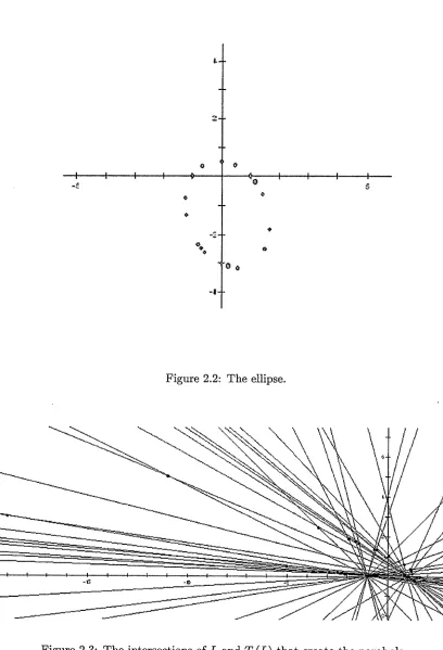
Next graph each of the equations L and T (L} respectively and identify their intersections,

and the locus of intersections will create an ellipse. See Figure 2.1 and 2.2.

Case 2: The Parabola

Let a = 4, b = —10, c = 1, d = 12 and r = 1,

P

so r (1 + a) and q 5

rc

1

and the m atrix T =

/ 4 -1 6 5 \

1 12 1 o i y

The m atrix of T 1 is

12 16

64 64

z T A

64 64

so T~

- l

y \ l )

16 1 4

z i i A

64 16

0

V o

o

i y

\y

16

X 64

/ 1 \ i - i \

0 = 0

V i ) I 1 )

64 X 16 J* 64

T

i x \

y

V 1 /

satisfies L through P (—1,0). So T (L}\

y = m(a; + l)

+ + + H + 1)

^y - i my

^ m x + ± x -

±

-i-X i£i

1 2 m + l — 1 2 m —1

n I — 64 np _| _ 64____

tZ 1—4m •** * 1 —4m

16 16

, , _ 1 2 m ± l _ 1 2 m ± l

" 4 —1 6 m '7' 4 —16m

1 2 m + l

4 —16m (a; - 1).

Substitute for m from line L into T (L) to find the equation of the conic,

T { L ) \ y 12( 4 r ) + ! ( ® - l )

y x

16 "

X +

W y

_2Z_

2—1 4_16JL> + 4_x+1

y _ 1 2 y + a + l

x —1 4 a;+ 4 —16?/

y (4x + 4 - 16y)

—2y2 — 3xy — 3y

4xy + 4y — 16y2

x 2 + 8xy + 16a/2 — 16a/ — 1

is the equation of the parabola.

(a; — 1) (12y + x + 1)

—2xy + 3a;2 + 3x + 2y — 3x — 3

12xy + x 2 + x — 12y — x — 1

0

Ln : y = m (x + 1 ) - > T ( L n) : _{y =} 1 2 m + l ( 4 —16m

Lx : y = x + 1 - > T ( L i ) : _{y =} _ 1 3 _{1 2 ^} , 13₁₂

L 2 : _{y = 2a; + 2} - > T ( L 2): _{y =} _ 2 5 _{28 x} , 25₂₈

L s : _{y =} 3a; + 3 - > L ( L 3): _{y =} _ 3 7 „ , 37 _{44 x 44}

Z 4 : _{y =4a; + 4} - > T ( L 4): _{y =} _ 4 9 „ , 49 _{60 x 60}

L 5 : _{y = —x} — 1 - > T ( L 5): _{y =} - I l _{2 0 J '} + 11 ₂₀

L 6 : _{y =} —2a; — 2 - > T ( L 6): _{y =} _ 2 3 _36x + 23₃₆

l

7 -.

L s : y = ~ ^ x ~ i - > T ( L 8): _{y =} _ _{1 2 ^} l s + _L ₁₂

L

:

L w ■ y = - k x - I

6 'l 6 T ( L 10) : y = ____i— 5L

Lxi : y = _ i T _ i &x 8 -> T ( L U ) : y = _ i a ; + J _ 12"" 12

L l 2 '• _{y =} - i a ; - - i- _{1 2 x 12 -> T ( L 12) : y = 0.}

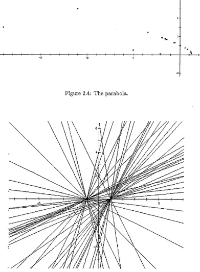
The locus of intersections will create a parabola. See Figure 2.3 and 2.4.

Case 3: The Hyperbola

Let a = 3, b = —2, c = 3, d = — 5 and r = 1 so p = 4 and q — 3

( 3

3 the matrix T =

\ 0

—2 4 \

- 5 3

0

The determinant 5 = — 9 and trace r = - 2 so r 2 > 4J and the conic is a hyperbola.

/ -1 \

0

V 1 / / 1 \

0

V 1 /

{ x \

y

\ i y

so T~-l

T - i

y =

\ 1 J

5X =2 _ 1 4 \

9 'L 9 y 9

iy

satisfies L through P (—1,0). So T (Z):

y = m (a; + 1)

x — jy — j = f a x —f a y

~ l y + j w :

( - | + |m ) y =

f a x — f a —

jm + j

3—5m \ 0 0 1 7

¥

7

x

1 i 2 " f " 1 2

-+ £ m - j + jm

3 ' 9

5 m —3 3 —5 m

__2__ m _L ___9__

2 m —3 ~ 2 m —3

5 m —3 - _ 5 m —3

2 m —3 2 m —3

T ( Z ) : _ 5 m —3_{2 m —3}5 4 ( z - l )

T ( L ) : 5 ( 4 i ) ~ 3

2(

+

)—

3

( z - l )

_ a _ £ —1

$2___3 s + i ° -22!— 3

aj+l °

4 _ X —1

5 y —3 x —3

2 y - 3 x —3

y (2y - 3x - 3)

2y2 - Zxy - 3y

= (a; — 1) (5y — 3x — 3)

= 5a;y — 3a;2 — 3a; — 5y + 3a; + 3

3a;2 — 8a;y + 2y2 + 2y — 3 = 0

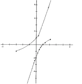
is the equation of the hyperbola. Graphing the conic in this case yields the following

equations,

Ln : y = m (x + 1 ) -4- T ( i n ) : _{y =} 5 m —3 ( _2m-3

Z i : _{y = x} + 1 4 i ( i l ) : _{y = 2a; — 2}

i 2 : _{y = 2# + 2 4} T ( i 2 ) : _{y = 7x - 7}

L 3 : _{y =} 3a; + 3 i ( i 3 ) : _{y = 4a; — 4}

i 4 : _{y = 4a; + 4} 4 i ( i 4 ) : _{y =} 17™ _{5 ®} 17₅

l

5 -.,

5 ® 5

L 6 : _{y =} -2a; — 2 4 T ( i e ) : _{y =} 13™ 13

7 ® 7

L 7 : _{y =} —3a; — 3 4 T ( i 7 ) : _{y = 2a; - 2}

i s : _{y = —4a; — 4} - 4 i ( i s ) : _{y =} 23™ 23

n ® l i

i 9 : _{y = ~ \ x - i} 4 i ( i 9 ) : _{y =} 11™ _ l i_{8 x 8}

i i o : _{y =} 4 i ( i i o ) : _{y = l x _} I

4® 4

i n : _{y =} 1 - + i_{4 ® + 4} 4 r ( L , i ) : _{y = 10®} 7 7₁₀

i l 2 : _{y =} _ 1 T _ 1

4® 4 4 i ( i l 2 ) : y = 17 14® _ 1714

i l 3 : _{y =} - 2 - a ; 4 - - i

16 ® 16 4 i ( i i 3 ) : y = _L™ 10® 101

i l 4 : _{y =} 15™ , 15

32® 32 4 i ( i l 4 ) : y = 22® 7 722

i

j.

G 0

+•

,■£

•>

4-$ ©

$

♦

©

-1

Figure 2.2: The ellipse.

-15

Figure 2.4: The parabola.

t

e

4--- &

Chapter 3

Hyperbolic Plane

Non-Euclidean geometry was one of the most momentous mathematical discov­

eries of the 19th century. Hyperbolic geometry is a non-Euclidean geometry which obeys

all the Euclidean postulates except the parallel postulate [Ped88]. In Hyperbolic geome­

try, the Poincare disk model, also called the conformal disk model, is a model in which

points of the geometry are in the open unit disk 5?. The lines of the geometry are seg­

ments of circles (arcs) contained in the disk orthogonal to the boundary circle C and this

also includes diameters th at are orthogonal to the disk.

Choosing two points P and Q in the hyperbolic plane, a transformation T such

that T (P) = Q is now a conformal hyperbolic transformation T which takes the pencil

of circles through P to the pencil through Q. Every direct non-Euclidean transformation

can be described as a Mobius transformation of the form:

where M < 1. |a|

The matrix associated with the transformation is

G T

This transformation leaves orientations unchanged and is called a direct non-Euclidean

transformation [BEG99]. A direct transformation is called: a rotation if T has a fixed

point in 2D, a translation if T has no fixed point in 2? but two distinct points on C, and

The direct transformation above results in the following theorem:

T heorem 3.1. A direct non-Euclidean transformation T can be written in the form

T (z) = K where K and m are complex numbers with — 1 and |m| < 1.

This is the canonical form of a direct non-Euclidean transformation [BEG99]. Note that

the transformation T with m = —R will map the point —R of £) to the origin. By two

applications of the theorem, we can obtain the general form of a direct non-Euclidean

transformation th at maps —R to R in 2). Let Ti (jz) be the transformation th at takes —R

to the origin and T2 (z} be the transformation th at takes R to the origin, so

and T2 (a) = K 2f = ^

the matrices th at are associated with the above transformations are

K 2 - R K 2 \

R 1

J

The inverse of A 2,

Kr R K X

- R 1

A, =

A₂- 1 1 R

- R K 2 k

2

so

1 R \ I K r RK±

- R K 2 K 2 I { - R 1

and let K \ = K — 2 K - R 2 R ( K + 1)

- R ( K + l ) - R 2K + \

Hence any direct transformation th at maps — R to R may be written in the form

T ( ; z ) (K - R 2) z + (R K + 1)

—J ? + 1 ) £ + (~ R ? K + 1 )

Thus, in correspondence with |A”| = 1, there are an infinite number of transfor­

mations th at take —R to R. First, we will dispense of the trivial case. Let T \ =

( c d \

and T2 = I I where T2 (0) = R.

= R and T , = f =

—aR + 6 = 0 d = Rc

b = aR

2x a aR

aR a

T2

c Rc

Rc c

t

2

,

Rc c

a Ra

Ra a

ac + R?ac R (ac + oc)

R {ac + ac) R 2ac + ac

ac + R 2ac 0

0 R 2ac + ac

i (1 - R 2) 0

0 i (R 2 —1)

1 0

0 - 1

which takes — R to R. This is nothing more than multiplication by —1 which takes the

real number line and maps it to itself. This case will result in a degenerate conic, which

Next, we will find a single parameter t where every value of t will generate a

different conic. Let R = tan h p and p = 5 where is the distance from the origin. If we

assume th at ac 7^ ai, then

T2T l =

ac+ R 2ac R{ac+ac)

1

1

a c+ R 2ac R(ac+ ac)

and since R — tanh ,

a c + R 2ac _ o c + ta n h 2 f Sc

2 # 2 ta n h

1 + ta n h 2 4 • ( l —t a n h 2 4 L a c

__ ____ J:__________ & f

2 ta n h j 2 ta n h ~ a c

But ■

1j',tan\ 2

g-2 °c

substitut-2 ta n h | 2 ta n h j - a c ’

coth d + it 1

2 ta n h j - a c

ing we get c o th d + ii. This is the desired transformation T =

that takes —R to R.

coth d — it

coth d + it

1

1 \

, the conic coth d — it /

that is produced by the correspondence between P (~ R ) and Q (R) is determined by t,

so the conic is determined by coth d + it where p and t will determine whether T is a ro­

tation, translation, or a limit rotation. In each case we must solve for the fixed points of T: Given the above transformation T =

(co th d + i t ) z + l

z 4-(co th d —it)

z 2 + (coth d —it) z = (coth d + it) z + 1

then z 4 i2+ 4

= it ± V l - t 2

so z\ = it + a/1 — t 2 and z? = it — \ / l — t 2. When |t| > 1 we get a rotation, if |t| < 1 a

translation, and when t = ±1 we will get a limit rotation [Sch79].

Lines in the hyperbolic plane are circular arcs orthogonal to the unit circle. If we

let H = | _ @ ] then the determinant of H = ad —

p d

| and if the determinant H < 0,

1 coth d + is

coth d — is 1

= 0

= 0

= 0

= 0. 1 coth d + is

coth d — is 1

then H will represent a circle. For example, let H =

then

G l )

( z + coth d — is z (coth d + is) + 1

z z + (coth d — is) z + (coth d + is) z + 1

|^|2 + 2 [z (coth d + is)] + 0

Let z = x + iy, then from the above equation:

a:2 + y2 + 2 (a: coth d — ys) + 1 = 0

x 2 + (2 coth d) x + y2 — 2sy = —1

(x + coth d)2 + (y — s)2. = — 1 + coth2 d + s2.

The center of the circle is (coth d, s) and the radius of the circle is v c o th 2 d + s2 — 1. So

any line in the Poincare plane is in the form of ( _ @ | , where 1/31 > 1 and I

V 1 / v 0

A line T, th at runs through —R can be represented by the following Hermitian

matrix,

coth d + is

for some s.

H =

coth d — is 1

If we let s = 1? ^- cot 8, then

H — 2R sin 0 (l + R 2) sin 8 + i (l — A2) cos 8

(l + A2) sin 8 — i (l — A2) cos 8 2R sin 8 , 0 < 0 < 7T

and

( - « 1 ) * ( - * )

= 0

R 2 (27?sin 0) — 2R (l + A2) sin0 + 2 Rsin# = 0

2 R sin 0 (R 2 — 2R + l) = 0

R 2 - 2R + 1 = 0 .

But R = tanh , so by substitution in the above equation, is equal to the following:

tanh2 5 — 2 tanh ^ + 1 = 0. The lines through R are represented by

y — cothd above, then

IS

— coth d + is

1 , for some s. If we use the same s = l —R 2

2R cot 6 as

H = 1

H =

( l + A2) sin0 — i (l — A2) cos6> 2R sin 8

and then by using the previous calculation from above 0 will

result in the same equation, tanh2 5 — 2 tanh ^ + 1 = 0.

Recall th at inversive geometry considers lines and circles in the plane to be the

same objects by adjoining the point 00. The inversive transformations form a group T

complex conjugation [Sch79]. We can now compute the image of a circle C under the

action of inverse transformations. If H is the Hermitian m atrix of the circle C we have

ZH Z* = 0, where Z — z 1 ) • We want a m atrix H such th at T (z) is on the line

represented by H , so ( T (F) 1 ) H = 0. If T + represents the transpose

of T , then this implies th at Z T +H T Z + = 0 and so (T+ )_1 H (T1) -1 is the Hermitian

matrix H of the circle T(C'). Note that (T+ )_1 = Tco, the cofactor m atrix of T , and

(T) 1 = T*o (the cofactor conjugate). This proves the following:

T heorem 3.2. I f H is the Hermitian matrix of the circle C and T is the matrix of a

LFT, then TC0H T f0 is the Hermitian matrix o f T (C).

The m atrix TroH T fo is called the spin conjugate of H by T . This spin action is the

principal method of transforming circles in C.

If H is in the pencil through P, then the image T (77) is as follows:

Let

T =

H =

Tco —

r p * ^CO

coth d + it 1

1 coth d — it

1 coth d + is

coth d — is 1

coth d — it —1

—1 coth d + it and

coth d + it —1

—1 coth d —it

s o T ( f f ) = T coH T t_co*

coth d —it —1 / 1 coth d + is \ coth d + it —1

We want to change the parameter t similarly to the change of s. These simple parameter

changes create all the hyperbolic rotations about —R to R. So let s = cot Q and

t = R2 ^ cot then

T = coth d + it 1

1 coth d —it

becomes

T = (l + R 2) sin — i (l — 7?2) cos 2R sin £

27? sin (l + 7?2) sin + i (l — 7?2) cos |

where 0 < (f) < and T (77) = TC0HT*0, where

Tco —

(7?2 + l) (sin + i (l — 7?2) (cos _-27?sin^

—27? sin (7?2 + l) (sin — i (l — 7?2) (cos

77 = 27? sin 0

(l + 7?2) sin 6 — i (l — 7?2) cos 6

(l + 7?2) sin# + i (l — 7?2) cos 0

2R sin 0

rp * ± C0

(7?2 + l) (sin — i (l — 7?2) (cos

—27? sin ^

—27? sin

(7?2 + l) (sin — i (l — 7?2) (cos

a b

c d

so, T (77) = , where

a = 27? sin (0 + ,

b = — (R 2 + l) sin (0 + + i (7?2 — l) cos (0 + </>),

c = — (7?2 + l) sin (0 + (ft) - i (7?2 — l) cos (0 + </>), and

Chapter 4

Spinor Correspondence

We now have representation of every line through — R = — tanh and a descrip­

tion of every direct isometry that takes —R to R. We can now find the conic determined

by the locus L n T (L).

However this locus will be complicated to find so we will simplify our work by

finding instead the locus of intersections of chords obtained by dilating these lines by a

hyperbolic factor of 2. Thus we reduce our work to a corresponding affine conic obtained

as in the previous chapter.

The radial dilation of the arcs through —R transforms the arcs into chords

th at share the endpoints on the boundary circle C. Previoiusly we let R = tanh and

d ( - R , R) = d. When we dilate by the hyperbolic factor of 2 we get ~

tanh d. This will dilate the entire pencil of lines through —R to chords th at go through

the point and can be written as the following theorem.

T heorem 4.1. I f the Hermitian matrix @ J represents a Poincare line for some /3,

with |/?| > 1, then the corresponding dilated chord with the same endpoints is represented

0

Proof:

Let R e10 be any point on f _ @ | . We want to show th at , e10 is on f @

P 1

+

m i i f

o

( R ei0 + P, PReie

+ 1 )

I

(Rei0 + P) Re~i8 + p R ei0 + 1 = 0

R 2 + pR e~ie + p R eie + 1 = 0

~P^e~i0 + P ^ e *

+ <±I =

o.

Then multiply by 2,

We need to check,

^ P e ~ i6 + ^ P e id

o £ 1 I

P

( 1 )

, x I

M *

lJ& I(S e « + 2 ) 1+* _{= 0}

I > ^ + I > ^ + 2 = 0,

so indeed 1^ 2 e10 is on 0

P

P

Recall th at if the straight line L through (—R, 0) is given by y = m (x + R) and

A is an affine transformation (—R, 0) to (R, 0), with linear part

A (L) is given by

a b

c d

, then the line

If the hyperbolic line through — R = — tanh 5 is represented by a Hermitan matrix

2R sin 6

H =

dilates to the chord through —1^ 2 with slope m = tan 0 represented by

(1+.R2) , , ( l - / J 2)

2 R + ? 2 R C° t ® 0

(a±g!) c o tg 2 R 1 2 R CUb(7

Then T (H) = I where, V “ /

a = 2R sin(0 + ^>),

b — — (R2 + l) sin (0 + </>) + i (R 2 — l) cos (6 + (/>'), and

b — — (R2 + l) sin ($ + </>)— i (R2 — l) cos (0 + <^>)

dilates to a chord through x^ - 2' with slope M = tan (# + <•/)).

. We can now find an affine transformation A th at takes chords through —R to

chords through R in correspondence with the action of T on the hyperbolic lines, by

determining constants a, b, c, d. Since M = then

tan (0 + <j>)

c + d ( C T ) ta n g

A = 1

jrjjy tan <?!>

|z + |t a n 0

1

When we take the determinant 8 = tan 2 (p + 1 — sec2 (p, and trace t — 2, then

t2 — 45 = 4 — 4 sec2 <p < 0

= 4 (l — sec2 <^>) < 0, if cp 7^ 0.

Thus, the resulting dilated conic determined by the locus of intersection is always an

ellipse.

Note th at if transformation T is an opposite isometry then the image of a line

through —R is obtained by complex conjugation followed by a direct transformation.

Since the Hermitian m atrix of the complex conjugate of a line is represented by the

transpose of the Hermitian m atrix of the line we only need to replace 9 with —9 to obtain

the Hermitian m atrix of the image line, whereby the slope of the chord after dilation is

M = 1^5- tan {cp — 9). Thus we find the affine matrix A from the equation

1 ^ - tan (<p - 0) 1 + f l 2 ta n 0 —ta n 9 1—K 2 1 + ta n <j> ta n 9

c 4 ~ t / t a n 9

a+^i1+o2_{1 —} tan 0 ’

this yields

1

| ^ ^ t a n ^

A —

- 1

The determinant 6 = — tan 2 (p — 1 = — sec2 <?!>, and the trace r = 0, so t2 — 4<5 — 4 sec2 (p >

0. Thus the opposite case of the dilated conic determined by the locus of intersection

always results in a hyperbola. So with r =

y2^

y - = 0

becomes

J?2 + l 1 - J?2

which simplifies to

x 2 — 2xy cot </> — 1 — R 2 -R2 + 1

4I22

(R 2 + 1) (1 - R 2)

x 2 cosh d — 2xy cot (f> — y 2 (tanh d) (sinh d } . coshd

Since this hyperbola is symmetric about the center of the disk it can always be rotated

about the origin into standard position and there are four distinct intersections with the

boundary circle C. This yields the following opposite case.

Opposite Case

If we let R = r; and (f> = | , then

tf 2 + l

1 — R 2 x 2 — 2xy cot <^> —

1

4R,2

(R 2 + 1) (1 - R 2) 0

simplifies to

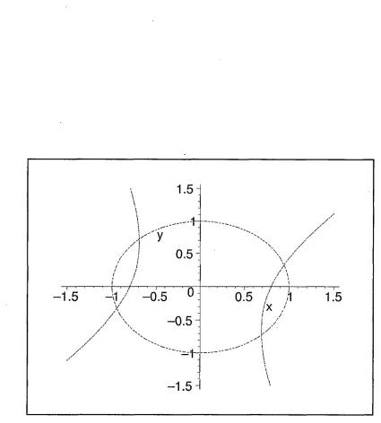
25a;2 — 10\/3a;y — 9y2 — 16 = 0. See Figure 4.1.

We can contract the equation of the hyperbolic conic by substituting u = _{x ~T~y} 2:E2 , . , v =

-h i'

a;2+2^ +1

x 2 cosh d — 2xy cot </> — y 2 — —- = (tanh d) (sinh d) coshd

which results in the following equation

4 co sh (/n 3 ) \ 2 _ f 8-^/3 \ _ f ___________4__________ A 2

(a:2+ i/2+ l ) / X \ 3 ( a : 2+2/2+ l ) J X ^ \ (co sh (/n 3 ))(a:2+7/2+ X )2 J — tan (Zn3) sin (Zn3) 0.

Figure 4.2 is the graph of the equation above combined with the graph of the hyper­

Chapter 5

Classification of Hyperbolic

Conics

The previous work shows that there are potentially six types of hyperbolic conics

(as opposed to the three types of affine Euclidean conic). Recall in the Euclidean affine

plane we consider three cases:

1) Ellipse, if the line at infinity is an exterior line,

2) Parabola, if the line at infinity is a tangent,

3) Hyperbola, if the line at infinity is a secant.

In the hyperbolic plane the line at infinity is replaced by the unit circle £. So the type of

conic is determined by the way this circle intersects the locus. Since these intersections are

the same for the dilated conic we only need to consider the number of ways an ordinary

Euclidean conic can intersect the unit circle.

Let’s consider our dilated ellipse in standard form

(1+fi2)2 x2 , ^~R2Y (v

4K 2 csc2 </>x 4 K 2 esc2 $

2Rcot<j>\2

1 - f t 2 ) ~

For 0 < <j> < 7r we have csc^ > 0, so the vertices of the ellipse on the major axis

(imaginary axis) are located at cot ± esc (f>. In particular, the upper vertex

following six cases:

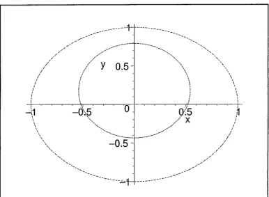
Case 1: No Intersection

If cot 2 < 1 and tan | < 1 and we let R = j and <j) = then

G + f l 2) 2 2 , ( 2 1 - f l 2) 2 ( _ 2 f l c o t 0 \ 2 _ b p r O T n p s 867 2 , 675 ( _ _8 / o \ 2 - 1

47Z2 csc2 </>® + 4-R2 esc2 </> \ V 1 - f l 2 J ~ 1 D e c o m e s 2 56® + 256 \ V 45 v 6 ) ~

See Figure 5.1.

Case 2: Unique Intersection; A Single Tangent

If cot < 1 and tan | = 1, or cot | = 1 and tan < 1 and we

let R = 2 — y/3 and <p = , then^

3a:2 + j (y — | ) 2 = 1. See Figure 5.2.

+ 4fl2*X (? ~

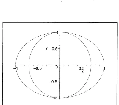
Case 3: Two Intersections; Both Tangents

If we cot 2 ~ 1 and 1 ^ 2 tan = 1. For example, let R = y/2 — 1 and cj> = then

+ (y - = 1 becomes 2a:2 + y2 = 1. See Figure 5.3.

Case 4: Two Intersections, A Secant

If y ^ ? cot < 1 and y ^ - tan | > 1, or y ^ - cot | > 1 and y ^ - tan | < 1 and we

let E = b and «/> = | , then (y - = 1 becomes

Case 5: Three intersections, A Tangent and A Secant

If

j2^2

iet R - and 0 = j , then ^ ^ x ? + 4^ c* 2\ (y - = 1 becomes

x 2 + j (y — l ) 2 = 1. See Figure 5.5.

Case 6: Four Intersections, Two Secants

If cot > 1 and tan > 1 and we let R = and <^> = J , then

■ , . . ( j - g 2 ) 2. _ 2 f l c o t # V _ x b e c o m e s 169 2 , _25_ ( _ 4 /q\ 2 _ i

4R?cs<?lj> 4 K 2 esc2 <j> \ y X-R2 J ~ 1 D e c o m e s 1 9 2 x + 192 \R ~ ■*"

See Figure 5.6.

Note: The equation of the ellipse can be written in terms of distance between the two

original points in the hyperbolic plane, d; and the angle of rotation </> th at determines T.

The equation of our dilated ellipse becomes

1

((tanh d)(csc0)) - X ((sinh d)(csc0))' (y — (sinhd) (cot d>))2 = 1,

where R = tanh i and

. 2g2

tanh j

2 1—ta n h |

To find the actual hyperbolic conic suppose th at the m atrix a b

c d produces the

Cartesian conic f e ^ z 2 + =

1-Since this conic is the result of dilating the hyperbolic conic, we can obtain the equation

of the hyperbolic conic by the usual inverse transformation procedure, th at is, if (x, y) is a

point on the hyperbolic conic then the dilation of (a;, y) must satisfy the above quadratic.

The dilation of (a:,y) is

1+X y 2)' S°’ if W® let U = A * and v = 1+Xy2

then the above equation results in the following

(i+a2) \ 2 , ( l - f l 2 ) 2

4 f l2 csc2 e U + 4 K 2 CSC2 </>G - 2 R_{l-R 2} cot 4> - 1 = 0

and becomes,

^ x 2 (sin2 </>)

(J2* ^ 1)2

which simplifies to the biquadratic or quartic form

+ (r2 + l) y -| (cot <j>) (l - B 2) — r2 (i?4 + l) + 4y2 + 1 = 0

where r 2 = x 2 + y 2 and R = tan 5.

If we use polar coordinates, x = r cos 9 and y = r sin (9, the above equation simplifies into

r 4 + A r3 + B r 2 + A r + 1 = 0.

This is the polar equation of the contraction to the hyperbolic conic, where

A = 2 ( i z ^ W sine = i « g sin(,

= 4 (cot (cschd) sin 0

B — — (7?4 — AR2 sin2 9 + l) = — (tanh2 p — 4 sin2 9 + coth2 p)

= 4sin2f l - 2 1+cn°s^ = —2 (cos29 + 2csch2d)

The symmetry in polar coefficients results from the fact tht the curve must be invariant

under the interchange of r with meaning that the curve is invariant under inversion

in the unit circle. The portion of the curve outside the unit circle results from the locus

of second intersections of the circular arcs through —R and R. We will now use the

Case 1: No Intersection

Let A = 2 ^ ~ R^ cot</> sin0, B = - ^ (fl* _ 4J?2 sin2 0 + i ) , j? = | , and

then r 4 + A r 3 + B r 2 + A r + 1 = 0 becomes

r 4 + |\ / 3 (sine) r3 + (4 sin2 0 — ^ ) r 2 + |\ / 3 (sine) r + 1 = 0. See Figure 5.7.

Case 2: A Unique Intersection; A Single Tangent

Let A = 2 gine, B = - ^ (R 4 - 4R2 sin2 0 + l ) , R = 2 - and </> = f ,

then r 4 + A r 3 + B r 2 + A r + 1 = 0 becomes

r 4 + 4 (sine) r 3 + (4 sin2 0 — 14) r 2 + 4 (sine) r + 1 = 0. See Figure 5.8.

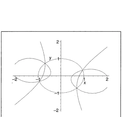
Case 3: Two Intersections; Both Tangents

Let A = sin0, b = (B4 - 4A2 sin2 0 + l) , R = ^ 2 - 1, and <f> = f , then r 4 + A r 3 + B r 2 + A r + 1 = 0 becomes r 4 + (4 sin2 0 — 6) r 2 + 1 — 0.

See Figure 5.9. Notice th at if we change to Cartesian coordinates this graph is a picture

of two circles intersecting on the boundary and has Cartesian factors of

(a;2 — 2x + y 2 — l) (x2 + 2x + y 2 — l) = 0 .

Case 4: Two Intersection; A Secant

Let A = sin#, B = (R4 - 4A2 sin2 0 + l) , R = i , and </> = f ,

then r 4 + A r 3 + B r 2 + A r + 1 = 0 becomes

Case 5: Three Intersections; A Secant and A Tangent

Let A = sinO, B = - (A4 - 4A2 sin20 + l ) , R = and <f> = f ,

then r 4 + A r 3 + B r 2 + A r + 1 = 0 becomes

r4 + | (sin 0 )r3 + (4 sin2 0 — r 2 + j (sin#) r + 1 = 0. See Figure 5.11.

Case 6: Four Intersections; Two Secants

Let A = 2^X R^ cot^ sin0, B = — (R 4 — 4A2 sin26 + l) , R = j , and (/> —

then r4 + A r 3 + B r 2 + A r + 1 = 0 becomes

Chapter 6

Conclusion

In this body of work, we have studied and shown how conics arise in planar

geometry as a linear correspondence between two concurrent pencils. The locus of inter­

sections L Pl T (L), as L runs through the entire pencil of lines through a point P, and

where T is an affine transformation such that T (P) = Q, creates an affine conic: an

ellipse, a parabola, or a hyperbola.

When we determined the intersection of L with T (L) we found the following

equation of the affine conic,

ex2 + (d — a) x y — by2 — (a + d )ry — cr2 = 0.

The type of conic was determined by the invariants of T , the determinant and trace of

the linear parts of the matrix T. This led to three cases of the affine conics.

We used this affine result to explore conics in the hyperbolic plane using Poincare’s

conformal disk model, where the lines of the geometry are segments of circles contained

in the disk orthogonal to the boundary circle £. We then chose two points P and Q and

a transformation T which takes the pencil of circles through P to the pencil through Q.

The transformation T is a linear fractional transformation th at preserves the disk.

We finally showed th at the conic produced by T is mapped to an affine conic

when dilation about the center of the disk by a hyperbolic factor of two is imposed. This

dilation takes the arc to chords of the disk th at share the same boundary points and

gives rise to a map, called the spinor map, th at allows us to classify the hyperbolic conic

by examining it’s affine counterpart. Since the affine conic is always an ellipse, we were

boundary of the disk. This resulted in six cases and the actual hyperbolic conic can be

Bibliography

[BEG99] David A. Brannan, Matthew F. Esplen, and Jeremy J. Gray. Geometry. Cam- 0

bridge University Press, Cambridge, 1999.

[Ped88] Dan Pedoe. Geometry. Dover Books on Advanced Mathematics. Dover Publi­

cations Inc., New York, second edition, 1988. A comprehensive course.

[Sar03] John Sarli. Polar inversion and conics, pages 1-17, 2003. Unpublished Exposi­

tory Work.

[Sch79] Hans Schwerdtfeger. Geometry of complex numbers. Dover Publications Inc.,

New York, 1979. Circle geometry, Moebius transformation, non-Euclidean

geometry, A corrected reprinting of the 1962 edition, Dover Books on Advanced