https://doi.org/10.5194/tc-12-3355-2018
© Author(s) 2018. This work is distributed under the Creative Commons Attribution 4.0 License.
Brief communication: Solar radiation management not as effective
as CO
2
mitigation for Arctic sea ice loss in hitting the
1.5 and 2
◦
C COP climate targets
Jeff K. Ridley and Edward W. Blockley
Met Office, Exeter, EX1 3PB, UK
Correspondence:Jeff Ridley ([email protected]) Received: 18 December 2017 – Discussion started: 3 January 2018
Revised: 7 September 2018 – Accepted: 14 September 2018 – Published: 23 October 2018
Abstract.An assessment of the risks of a seasonally ice-free Arctic at 1.5 and 2.0◦C global warming above pre-industrial levels is undertaken using model simulations with solar ra-diation management to achieve the desired temperatures. An ensemble of the CMIP5 model HadGEM2-ES uses solar ra-diation management (SRM) to achieve the desired global mean temperatures. It is found that the risk for a season-ally ice-free Arctic is reduced for a target temperature for global warming of 1.5◦C (0.1 %) compared to 2.0◦C (42 %), in general agreement with other methodologies. The SRM produced more ice loss, for a specified global temperature, than for CO2mitigation scenarios, as SRM produces a higher polar amplification.
Copyright statement. The works published in this journal are distributed under the Creative Commons Attribution 4.0 License. This license does not affect the Crown copyright work, which is re-usable under the Open Government Licence (OGL). The Creative Commons Attribution 4.0 License and the OGL are interoperable and do not conflict with, reduce or limit each other.
© Crown copyright 2018
1 Introduction
The 21st Conference of Parties (COP) to the UN Framework Convention on Climate Change held in Paris in 2016 made a commitment to limiting global-mean warming since the pre-industrial era to well below 2.0◦C and to pursue efforts to limit the warming to 1.5◦C (UNFCCC, 2015). The 1.5◦C
target reflects a threshold at which the likely local impacts of climate change are beyond the ability of society to cope with. This is especially applicable to the small island states that are susceptible to sea level rise, groundwater salinification, and loss of coral reefs. One such risk is the loss of Arctic sea ice, for which previous studies (Sanderson et al., 2017; Screen and Williamson, 2017; Jahn, 2018; Niederdrenk and Notz, 2018; Sigmond et al., 2018) used a number of methodologies with various climate models under CO2mitigation scenarios. The findings are broadly similar, showing that there is a low chance of an ice-free Arctic if global temperatures are limited to 1.5◦C and a moderate chance at 2◦C.
It has been suggested that geoengineering, otherwise known as solar radiation management (SRM), may be a stop-gap measure to halt these impacts, stabilizing Earth’s temper-ature at 1.5 K, before CO2mitigation can take effect (Chen and Xin, 2017). Here we evaluate the impact of SRM on Arctic sea ice decline and compare with mitigation methods alone, through the implementation of SRM, in our climate model HadGEM2-ES. We use the SRM strategy of strato-spheric aerosol injection, which mimics large volcanic erup-tions (Crutzen, 2006).
The impacts of a seasonally ice-free Arctic include in-creased ice loss from Greenland (Day et al., 2013; Liu et al., 2016), and hence sea level rise, and may contribute to extreme weather events in the northern mid-latitudes (Over-land et al., 2015; Francis et al., 2017). Furthermore, storms and waves in the open water may cause coastal erosion, im-pacting marine ecosystems, infrastructure, and local commu-nities (Steiner et al., 2015; Radosavljevic et l., 2016).
With the objective to limit the increase in global average temperature to well below 2.0◦C above pre-industrial lev-els and to pursue efforts to limit the temperature increase to 1.5◦C above pre-industrial levels, we need to ascertain the costs of mitigation and associated climate risks. It has been suggested that SRM may be a means to reduce the im-mediate costs of climate mitigation, especially to reach the 1.5◦C target (Sugiyama et al., 2017). There have been a num-ber of proposed mechanisms to reduce the solar radiation reaching the Earth’s surface through geoengineering (Shep-herd, 2009; Ming et al., 2014). Here we employ the SRM methodology of increasing sulfate aerosols in the strato-sphere, which in the CMIP5 climate model HadGEM2-ES is achieved through uniformly increasing the number density of volcanic aerosols. This work expands on the methodology of Jones et al. (2018) in which SRM is applied in HadGEM2-ES. Although this method can stabilize global temperatures, it produces a spatial temperature pattern with overcooling in the tropics and slight warming at high latitudes (Kravitz et al., 2017). This means it may be effective in reducing ice loss compared to doing nothing, as SRM cools everywhere, but not so effective compared with reducing greenhouse gas emissions. Here we evaluate this by comparing geoengi-neered 1.5 and 2.0◦C worlds with the equivalent-temperature
CO2-mitigated worlds. The use of modelled SRM in this pa-per does not endorse or advocate either testing or actual im-plementation of geoengineering. Our purpose here is to study and inform.
2 Method
HadGEM2-ES is a coupled atmosphere–ocean general circu-lation model with atmospheric resolution of N96 (1.875◦× 1.25◦) with 38 vertical levels and an ocean resolution of 1◦ at mid-latitudes (increasing to 1/3◦ at the Equator) and 40 vertical levels (Jones et al., 2011). The ocean grid has an island at the North Pole to avoid the singularity caused by a convergence of the meridians. The sea ice compo-nent uses elastic–viscous–plastic dynamics, five ice thick-ness categories, and zero-layer thermodynamics (McLaren et al., 2006). The HadGEM2-ES simulation produces a good representation of Arctic sea ice, thickness, trends, seasonal cycle, and variability when compared against observations (The HadGEM2 Development Team, 2011; Baek et al., 2013; Huang et al., 2017). Simulated temperature changes are ref-erenced against the mean global temperature from a 400-year
section of a pre-industrial control simulation with constant forcing at 1860 levels of greenhouse gases.
The objective is to explore several SRM scenarios branch-ing from the transient simulations of Representative Concen-tration Pathway (RCP) scenarios (van Vuuren et al., 2011). RCP scenarios start from the year 2005 and continue to 2100. The mean of the four RCP2.6 scenario simulations reaches a peak global mean temperature of+2◦C while that of RCP4.5 reaches+2.9◦C. Each scenario is allowed to develop with-out SRM adjustment until a global temperature of+1.5◦C is reached in RCP2.6 (year 2020) and +2.0 and +2.5◦C in RCP4.5 (years 2040 and 2060 respectively in the ensem-ble means). New simulations, using SRM, are started from these points using continuous injection of SO2into the model stratosphere between 16 and 25 km. This SO2is oxidized to form sulfate aerosols that reflect incoming solar radiation and thus cool the climate. As HadGEM2-ES does not have a well-resolved stratosphere, SO2is injected uniformly across the globe to reduce any problems with stratospheric transport. Since the global temperature of the RCPs varies in time, the SO2required to maintain a constant global temperature will also vary in time. The difference between the RCP ensem-ble mean and target temperatures (e.g. 2.0◦C), calculated at 10-year intervals, was used to determine the time profile of SO2injection in combination with calibration simulations to assess the amount of cooling for a given level of SO2 injec-tion (−0.115◦C Tg [SO2]−1yr−1). Provided the temperature differences are small, a single value for climate sensitivity to SO2may be applied. The same SO2time profile was injected into each of the ensemble members with the same target tem-perature.
For CMIP5 a historical+ scenario initial condition en-semble of four HadGEM2-ES members was completed. A larger ensemble is required to generate a probability distribu-tion of sea ice decline. To achieve this we take the four sepa-rate RCP ocean and atmosphere start conditions and intermix them (e.g. RCP ensemble member-1 atmosphere with RCP ensemble member-2 ocean) to provide 16 perturbed mem-bers for each start date of 2020, 2040, and 2060. The appli-cation of a random atmosphere to an ocean state equilibrates within a few days (Griffies and Bryan, 1997). The resulting ensemble spread in global mean temperature is larger than that for the initial four-member ensemble, indicating that the resulting initial perturbations are sufficient to generate a wide range of climate trajectories.
The ensembles analysed in this study are as follows.
– Ensemble 1 starts at 1.5◦C on RCP2.6 and levels out at 1.5◦C above pre-industrial control (1860).
– Ensemble 2 starts at 2.0◦C on RCP4.5 and levels out to 1.3◦C above pre-industrial control (1860).
2000 2020 2040 2060 2080 2100 Year
0 1 2 3
Global
temperature
(
C)
o
2000 2020 2040 2060 2080 2100
Year 0
2 4 6
Ice
extent
(km
x10
)
2
6
2000 2020 2040 2060 2080 2100
Year 0
1 2 3
Global
temperature
(
C)
o
2000 2020 2040 2060 2080 2100
Year 0
2 4 6
Ice
extent
(km
x10
)
2
6
2000 2020 2040 2060 2080 2100
Year 0
1 2 3
Global
temperature
(
C)
o
2000 2020 2040 2060 2080 2100
Year 0
2 4 6
Ice
extent
(km
x10
)
2
6
(a) (b)
(c) (d)
(e) (f)
Figure 1. (a)Global mean 1.5 m temperature and(b)Arctic sea ice extent for the four ensemble RCP2.6 simulations (black) and the 16-member Ensemble 1 initiated from+1.5◦C (red).(c)Global mean 1.5 m temperature and(d)Arctic sea ice extent for the four ensemble RCP4.5 simulations (black) and the 16-member Ensemble 2 initiated from+2◦C (red).(e)Global mean 1.5 m temperature and(f)Arctic sea ice extent for the four ensemble RCP4.5 simulations (black) and the 16-member Ensemble 2 initiated from+2.5◦C (red).
a
( ) (b) (c)
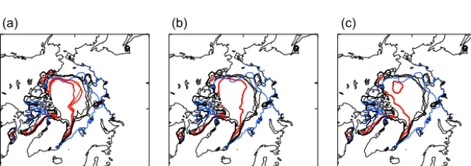
Figure 2.The spatial pattern of the sea ice edge (the 15 % concentration contour) with the observation mean for the period 2006–2015 from HadISST (Rayner et al., 2003) in blue, the four-member model RCP ensemble for the equivalent period in black, and the 16-member ensemble simulations for the mean of years 2080–2099 in red.(a)The RCP2.6 simulations and Ensemble 1;(b)the RCP4.5 simulations and Ensemble 2;(c)the RPC4.5 simulations and Ensemble 3.
3 Results
The September sea ice extent in the three ensembles (Fig. 1) remains stable in Ensemble 1 but recovers in Ensemble 2 and Ensemble 3. The recovery is in line with the downward drift in global mean temperatures as indicated by the reversibility and decadal temperature sensitivity of Arctic sea ice change (Ridley et al., 2012). The spatial pattern of sea ice edge (Fig. 2) shows that the model represents a low ice extent for
Ensem-ble 3 has members with discontinuous ice cover, with a patch of ice in the Beaufort Gyre, where the ice was originally too thick, and extending along the North Greenland and Cana-dian Archipelago coasts. That Ensemble 3 has a different spatial pattern of the ice edge, and yet is only a few tenths of a degree warmer than the other two ensembles at 2100, is associated with the 15 % threshold used to derive the ice edge. The summer ice cover in the central Arctic has an ex-tensive marginal ice zone and so the threshold definition of the ice edge at 15 % ice concentration is noisy.
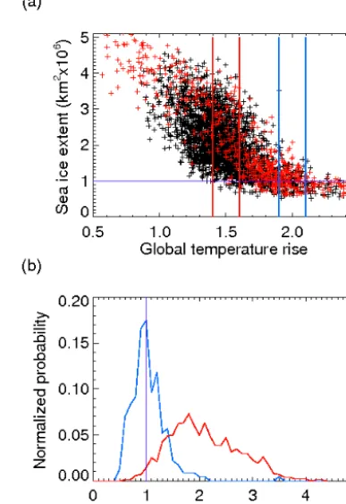
The time drift in September ice extent in Ensemble 2 and Ensemble 3 leads us to conclude that attempting to create a mean state for specific global temperatures, without pre-cise tuning of the SRM for each RCP, is not sensible. In-stead, all ensembles are combined to form a continuum of an-nual global temperature and September Arctic sea ice states. The scatter plot of all 48 ensemble members and 2880 sim-ulated years is shown in Fig. 3. It is expected that the use of SRM will change the regional energy budget, with many models showing an enhanced warming in the Arctic (Kravitz et al., 2017; Jones et al., 2018). To compare SRM and green-house gas scenarios for the same global temperature rise, in addition to the SRM ensembles, the data from the transient RCP2.6 and RCP4.5 is added to the scatter plot. The RCPs’ climate is moderated by greenhouse gas emissions, and so serve as a reference for the SRM ensembles. The data from the transient simulations show characteristics broadly sim-ilar to the ensemble members, with high scatter in sea ice extent at low global temperature and less at higher tempera-tures. However, it is evident that the RCP simulations show a marginally greater sea ice extent than for SRM, and we as-sess this through model polar amplification. The polar ampli-fication, as defined by1T(60–90◦N)/1T(global)(where1T is a
20-year time mean temperature rise – in this case a global rise of 1◦C), is 2.48±0.08 for the RCPs and 2.89±0.12 for the SRM ensembles. The higher polar amplification for the SRM case is in agreement with Kravitz et al. (2017). In principle, the higher SRM polar amplification should result in a faster decline of the Arctic sea ice, so we investigate if the sea ice extent is lower for SRM then RCPs at 1.5◦C. The mean sea ice extent in the temperature band 1.5±0.1◦C (Fig. 3a) above pre-industrial levels is 2.45±0.02×10⁶km2with SRM and 2.90±0.09×10⁶km2 in the RCPs (with CO2 mitigation). This result shows a higher sea ice loss in the SRM experi-ments than with mitigation at 99.7 % confidence.
The probability distribution function (PDF) is derived for sea ice extent within temperature bands: 1.5±0.1 (sample size 1068 of which 77 are RCP) and 2.0±0.1◦C (sample
size 341 of which 112 are RCP) above pre-industrial levels. The probability of a single year with an ice extent less than 1 million km2at+1.5◦C is 0.1 % and that at+2.0◦C is 42 %.
Figure 3. (a) All 48 ensemble members are combined to derive a September ice extent vs. global temperature scatter plot (black symbols) with the complete four-member RCP2.6 and four-member RCP4.5 simulations included (red symbols). The threshold of 1 mil-lion km2signifying an almost ice-free Arctic is shown with the pur-ple horizontal line. The data points used to evaluate the probability distribution function of(b)are selected from the global temperature thresholds of 1.5±0.1◦C (red vertical lines) and 2.0±0.1◦C (blue vertical lines).(b)The normalized probability distribution functions of Arctic sea ice extent at global temperature rises of 1.5±0.1◦C (red) and 2.0±0.1◦C (blue) are associated with the ensemble mem-bers shown in(a). The 1 million km2threshold for an ice-free Arctic is indicated by the purple vertical line.
4 Conclusions
a significant difference between SRM and RCP. In common with the studies of Haywood et al. (2013), Jones et al. (2017, 2013), and Trisos et al. (2018) our study provides another cautionary aspect for SRM implementation. These studies showed counterbalancing deleterious impacts on Sahelian drought and North Atlantic hurricane frequency if SRM were applied in a hemispherically asymmetric manner and a sig-nificant termination effect that ecosystems may not have the capacity to deal with should high levels of SRM be relied on. An increased localized SRM over the Arctic can reduce the albedo feedback but enhances other positive feedbacks from clouds and poleward heat transport. However, sufficient local SRM can halt sea ice decline (Tilmes et al., 2014). Here we show that SRM is not as effective as conventional mitigation in reducing Arctic sea ice loss, due to a higher polar amplifi-cation for SRM for the same amount of global warming.
Code and data availability. The source code for the model used in this study is available to use. To apply for a license for the UM go to http://www.metoffice.gov.uk/research/collaboration (last access: 22 October 2018). For more information on the exact model versions and branches applied, please contact the authors. Data from the sim-ulations are archived at the Met Office and available for research use through the Centre for Environmental Data Analysis JASMIN platform (http://www.jasmin.ac.uk/, last access: 22 October 2018); for details please contact [email protected] ref-erencing this paper.
Author contributions. JR designed the study, ran the simulations, and wrote most of the manuscript. Both authors contributed in in-terpreting the results and improving the text.
Competing interests. The authors declare that they have no conflict of interest.
Acknowledgements. The authors thank Jim Haywood and Jason Lowe for insight and advice.
Edited by: Xavier Fettweis
Reviewed by: three anonymous referees
References
Baek, H. J., Lee, J., Lee, H. S., Hyun, Y. K., Cho, C., Kwon, W. T., Marzin, C., Gan, S. Y., Kim, M. J., Choi, D. H., Lee, J., Lee, J., Boo, K. O., Kang, H. S., and Byun, Y. H.: Climate change in the 21st century simulated by HadGEM2-AO under represen-tative concentration pathways, Asia-Pacific, J. Atmos. Sci., 49, 603, https://doi.org/10.1007/s13143-013-0053-7, 2013. Chen, Y. and Xin, Y. : Implications of
geoengineer-ing under the 1.5◦C target: Analysis and policy
suggestions, Adv. Clim. Change Res., 8, 123–129, https://doi.org/10.1016/j.accre.2017.05.003, 2017.
Comiso, J. C., Meier, W. N., and Gersten, R.: Variabil-ity and trends in the Arctic Sea ice cover: Results from different techniques, J. Geophys. Res., 122, 6883-6900, https://doi.org/10.1002/2017JC012768, 2017.
Crutzen, P.: Albedo enhancement by stratospheric sulfur injections: A contribution to resolve a policy dilemma, Clim. Change, 77, 211–220, https://doi.org/10.1007/s10584-006-9101-y, 2006. Day, J. J., Bamber, J. L., and Valdes, P. J.: The
Green-land Ice Sheet’s surface mass balance in a seasonally sea ice-free Arctic, J. Geophys. Res.-Earth, 118, 1533–1544, https://doi.org/10.1002/jgrf.20112, 2013.
Francis, J. A., Vavrus, S. J., and Cohen, J.: Amplified Arc-tic warming and mid-latitude weather: new perspectives on emerging connection, WIRES Clim. Change, 8, e474, https://doi.org/10.1002/wcc.474, 2017.
Griffies, S. and Bryan, K. : A predictability study of simulated North Atlantic multidecadal variability, Clim. Dynam., 13, 459, https://doi.org/10.1007/s003820050177, 1997.
Haywood, J. M., Jones, A., Bellouin, N., and Stephenson, D. B.: Asymmetric forcing from stratospheric aerosols im-pacts Sahelian drought, Nat. Clim. Change, 3, 660–665, https://doi.org/10.1038/NCLIMATE1857, 2013.
Huang, F., Zhou, X., and Wang, H.: Arctic sea ice in CMIP5 climate model projections and their seasonal variability, Acta Oceanol. Sin., 36, 1–8, https://doi.org/10.1007/s13131-017-1029-8, 2017. Jahn, A.: Reduced probability of ice-free summers for 1.5◦C compared to 2◦C warming, Nat. Clim. Change, 8, 409–413, https://doi.org/10.1038/s41558-018-0127-8, 2018.
Jones, A., Haywood, J.M., Alterskjær, K., Boucher, O., Cole, J. N. S., Curry, C. L., Irvine, P. J., Ji, D., Kravitz, B., Kristjánsson, J. E., Moore, J., Niemeier, U., Robock, A., Schmidt, H., Singh, B., Tilmes, S., Watanabe, S., and Yoon, J.-H.: The impact of abrupt suspension of solar radiation management (termination effect) in experiment G2 of the Geoengineering Model Intercom-parison Project (GeoMIP), J. Geophys. Res., 118, 9743–9752, https://doi.org/10.1002/jgrd.50762, 2013.
Jones, A. C., Haywood, J. M., Dunstone, N., Hawcroft, M. K., Hodges, K., Jones, A., and Emanuel, K.: Impacts of hemi-spheric solar geoengineering on tropical cyclone frequency, Nat. Commun., 8, 1382, https://doi.org/10.1038/s41467-017-01606-0, 2017.
Jones, A. C., Hawcroft, M. K., Haywood, J. M., Jones, A., Guo, X., and Moore, J. C.: Regional Climate Impacts of Stabilizing Global Warming at 1.5 K Using Solar Geoengineering, Earth’s Future, 6, 230–251, https://doi.org/10.1002/2017EF000720, 2018. Jones, C. D., Hughes, J. K., Bellouin, N., Hardiman, S. C., Jones,
Kravitz, B., MacMartin, D. G., Mills, M. J., Richter, J. H., Tilmes, S., Lamarque, J.-F., Tribbia, J. J., and Vitt, F.: First simulations of designing stratospheric sulfate aerosol geoengineering to meet multiple simultaneous climate objectives, J. Geophys. Res.-Atmos., 122, 12616–12634, https://doi.org/10.1002/2017JD026874, 2017.
Liu, J., Chen, Z., Francis, J., Song, M., Mote, T., and Hu, Y.: Has Arctic sea-ice loss contributed to increased surface melt-ing of the Greenland ice sheet?, J. Clim., 29, 3373–3386, https://doi.org/10.1175/JCLI-D-15-0391.1, 2016.
McLaren, A. J., Banks, H. T., Durman, C. F., Gregory, J. M.,Johns, T. C., Keen, A. B., Ridley, J. K., Roberts, M. J., Lipscomb, W. H., Connolley, W. M., and Laxon, S. W.: Evaluation of the sea ice simulation in a new coupled atmospheric-ocean climate model (HadGEM1), J. Geophys. Res., 111, C12014, https://doi.org/10.1029/2005JC003033, 2006.
Ming, T., de Richter, R., Liu, W., and Caillol, S.: Fighting global warming by climate engineering: Is the Earth radiation manage-ment and the solar radiation managemanage-ment any option for fight-ing climate change?, Renew. Sust. Energ. Rev., 31, 792–834, https://doi.org/10.1016/j.rser.2013.12.032, 2014.
Niederdrenk, A. L. and Notz, D : Arctic sea ice in a 1.5◦C warmer world, Geophys. Res. Lett., 45, 1963–1971, https://doi.org/10.1002/2017GL076159, 2018.
Overland, J., Francis, J., Hall, R., Hanna, E., Kim, S., and Vihma, T.: The melting Arctic and midlatitude weather pat-terns: Are they connected?, J. Climate, 28, 7917–7932, https://doi.org/10.1175/JCLI-D-14-00822.1, 2015.
Radosavljevic, B., Lantuit, H., Pollard, W., Overduin, P., Couture, N., Sachs, T., Helm, V., and Fritz, M. : Erosion and Flooding-Threats to Coastal Infrastructure in the Arctic: A Case Study from Herschel Island, Yukon Territory, Canada, Estuaries Coasts, 39, 900–915, https://doi.org/10.1007/s12237-015-0046-0, 2016. Rayner, N. A., Parker, D. E., Horton, E. B., Folland, C. K., Alexan-der, L. V., Rowell, D. P., Kent, E. C., and Kaplan, A.: Global analyses of sea surface temperature, sea ice, and night marine air temperature since the late nineteenth century J. Geophys. Res.-Atmos., 108, 4407, https://doi.org/10.1029/2002JD002670, 2003.
Ridley, J. K., Lowe, J. A., and Hewitt, H. T.: How re-versible is sea ice loss?, The Cryosphere, 6, 193–198, https://doi.org/10.5194/tc-6-193-2012, 2012.
Sanderson, B. M., Xu, Y., Tebaldi, C., Wehner, M., O’Neill, B., Jahn, A., Pendergrass, A. G., Lehner, F., Strand, W. G., Lin, L., Knutti, R., and Lamarque, J. F.: Community climate simulations to assess avoided impacts in 1.5 and 2◦C futures, Earth Syst. Dy-nam., 8, 827–847, https://doi.org/10.5194/esd-8-827-2017, 2017. Screen, J. A. and Williamson, D.: Ice-free Arc-tic at 1.5◦C?, Nat. Clim. Change, 7, 230–231, https://doi.org/10.1038/nclimate3248, 2017.
Shepherd, J. G.: Geoengineering the climate: Science, governance and uncertainty (Policy Document No. 10/09), Royal Society, London, 82 pp., 2009.
Sigmond, M., Fyfe, J. C., and Swart, N. C.: Ice-free Arctic projec-tions under the Paris Agreement, Nat. Clim. Change, 8, 404–408, https://doi.org/10.1038/s41558-018-0124-y, 2018.
Steiner, N., Azetsu-Scott, K., Hamilton, J., Hedges, K., Hu, X., Janjua, M. Y., Lavoie, D., Loder, J., and Melling, H.: Ob-served trends and climate projections affecting marine ecosys-tems in the Canadian Arctic, Environ. Rev., 23, 191–239, https://doi.org/10.1139/er-2014-0066, 2015.
Stroeve, J., Barrett, A., Serreze, M., and Schweiger, A.: Using records from submarine, aircraft and satellites to evaluate climate model simulations of Arctic sea ice thickness, The Cryosphere, 8, 1839–1854, https://doi.org/10.5194/tc-8-1839-2014, 2014. Sugiyama, M., Arino, Y., Kosugi, T., Kurosawa, A., and
Watan-abe, S.: Next steps in geoengineering scenario research: limited deployment scenarios and beyond, Clim. Policy, 18, 681–689, https://doi.org/10.1080/14693062.2017.1323721, 2017. The HadGEM2 Development Team: G. M. Martin, Bellouin, N.,
Collins, W. J., Culverwell, I. D., Halloran, P. R., Hardiman, S. C., Hinton, T. J., Jones, C. D., McDonald, R. E., McLaren, A. J., O’Connor, F. M., Roberts, M. J., Rodriguez, J. M., Woodward, S., Best, M. J., Brooks, M. E., Brown, A. R., Butchart, N., Dear-den, C., Derbyshire, S. H., Dharssi, I., Doutriaux-Boucher, M., Edwards, J. M., Falloon, P. D., Gedney, N., Gray, L. J., Hewitt, H. T., Hobson, M., Huddleston, M. R., Hughes, J., Ineson, S., In-gram, W. J., James, P. M., Johns, T. C., Johnson, C. E., Jones, A., Jones, C. P., Joshi, M. M., Keen, A. B., Liddicoat, S., Lock, A. P., Maidens, A. V., Manners, J. C., Milton, S. F., Rae, J. G. L., Rid-ley, J. K., Sellar, A., Senior, C. A., Totterdell, I. J., Verhoef, A., Vidale, P. L., and Wiltshire, A.: The HadGEM2 family of Met Of-fice Unified Model climate configurations, Geosci. Model Dev., 4, 723–757, https://doi.org/10.5194/gmd-4-723-2011, 2011. Tilmes, S., Jahn, A., Kay, J. E., Holland, M., and
Lamar-que J.-F.: Can regional climate engineering save the sum-mer Arctic sea ice?, Geophys. Res. Lett., 41, 880–885, https://doi.org/10.1002/2013GL058731, 2014.
Trisos, C. H., Amatulli, G., Gurevitch, J., Robock, A., Xia, L., and Zambri, B.: Potentially dangerous conse-quences for biodiversity of solar geoengineering imple-mentation and termination, Nat. Ecol. Evol., 2, 475–482, https://doi.org/10.1038/s4155901704310, 2018.
UNFCCC: Adoption of the Paris Agreement, Report No. FCCC/CP/2015/L.9/Rev.1, available at: http://unfccc.int/ resource/docs/2015/cop21/eng/l09r01.pdf (last access: 12 October 2018), 2015.