www.nonlin-processes-geophys.net/14/59/2007/ © Author(s) 2007. This work is licensed under a Creative Commons License.
Nonlinear Processes
in Geophysics
Model error estimation in ensemble data assimilation
S. Gillijns and B. De Moor
SCD-SISTA-ESAT, Katholieke Universiteit Leuven, Leuven, Belgium
Received: 21 April 2006 – Revised: 8 January 2006 – Accepted: 8 January 2006 – Published: 31 January 2007
Abstract. A new methodology is proposed to estimate and
account for systematic model error in linear filtering as well as in nonlinear ensemble based filtering. Our results extend the work of Dee and Todling (2000) on constant bias errors to time-varying model errors. In contrast to existing method-ologies, the new filter can also deal with the case where no dynamical model for the systematic error is available. In the latter case, the applicability is limited by a matrix rank con-dition which has to be satisfied in order for the filter to exist. The performance of the filter developed in this paper is limited by the availability and the accuracy of observations and by the variance of the stochastic model error compo-nent. The effect of these aspects on the estimation accu-racy is investigated in several numerical experiments using the Lorenz (1996) model. Experimental results indicate that the availability of a dynamical model for the systematic er-ror significantly reduces the variance of the model erer-ror esti-mates, but has only minor effect on the estimates of the sys-tem state. The filter is able to estimate additive model error of any type, provided that the rank condition is satisfied and that the stochastic errors and measurement errors are signifi-cantly smaller than the systematic errors. The results of this study are encouraging. However, it remains to be seen how the filter performs in more realistic applications.
1 Introduction
Error in environmental forecasting is mainly due to two causes: inaccurate initial conditions and deficiencies in the model. Much of attention has focused on reducing the ef-fect of the first cause. Several suboptimal filters have been developed to assimilate measurements into large-scale mod-els in order to come up with a more accurate estimate of the
Correspondence to: S. Gillijns
initial condition. The ensemble Kalman filter (EnKF), intro-duced by Evensen (1994), has gained particular popularity for environmental state estimation thanks to its ease of imple-mentation and its robustness against filter divergence. Nowa-days, the number of data assimilation applications involving the EnKF is numerous, see (Evensen, 1994; Houtekamer and Mitchell, 2001; Reichle et al., 2002; Evensen, 2003) and the references therein.
However, apart from stochastic model uncertainties, the EnKF is based on a perfect model assumptions. It is thus not able to deal with deficiencies in the model, which may play a major role in environmental forecasting (Orrell et al., 2001). A number of authors have addressed this lack of the EnKF. The effect of systematic model errors on the estimation ac-curacy is investigated in (Mitchell and Houtekamer, 2002) and (Reichle et al., 2002). In (Mitchell and Houtekamer, 2002; Heemink et al., 2001), an ad hoc method is used to ac-count for systematic errors by treating the errors like random white noise with prescribed error covariance matrix. Another heuristic technique is covariance inflation (Anderson and An-derson, 1999), where the spread of the ensemble is artifi-cially enlarged to make the filter more robust against model errors. Although both methods are successfully used in prac-tice, they do not make use of the observations which con-tain information about the model error. Furthermore, none of both methods is able to yield estimates of the model error.
used for estimating systematic model error in ensemble based data assimilation as well as in variational data assimilation (Zupanski, 1997; Griffith and Nichols, 2000; Martin et al., 2002; Zupanski and Zupanski, 2006). The method has the advantage of being very flexible and being able to incorpo-rate different types of prior knowledge about the model er-ror into the assimilation procedure. However, the fact that a model which describes the dynamical evolution of the error must be available, limits the applicability of the method.
There are types of model error of which the dynamics are not known, for example certain types of time-varying bias errors, errors due to unresolved scales, discretization errors, unmodeled dynamics and unknown disturbances. In these cases, the state augmentation method can not be used.
Like (Dee and Da Silva, 1998; Dee and Todling, 2000), this paper addresses the problem of additive model error es-timation and correction in data assimilation. Based on the optimal linear filters of Kitanidis (1987); Gillijns and De Moor (2007), we develop a rigorous and efficient method to deal with systematic model error in linear filtering as well as in nonlinear ensemble based filtering. In case a dynamical model for the systematic error is available, our results extend the work of Dee and Todling (2000) to time-varying model error. More precisely, using the same approximation, we de-velop a suboptimal but efficient filter where the estimation of the time-varying model error and the state are intercon-nected. However, provided that a certain matrix rank condi-tion is satisfied, our method can also deal with the case where no dynamical model for the systematic error is available.
The performance of the filter developed in this paper is limited by the availability and the accuracy of observations and by the variance of the stochastic model error component. The effect of these aspects on the estimation accuracy is in-vestigated in several numerical experiments using the Lorenz (1996) model. Due to the limitations, the method can in prac-tice not be used to correct the entire state vector for all types of errors described above. However, it can be used to ob-tain, possibly for a limited number of state variables, an idea about the additive effect of the model error affecting these state variables, which is especially useful if the dynamics of the error are unknown. These estimates might give insight into the dynamics of the error, which might lead to a re-finement of the simulation model or to the development of a “model error model” which can then be incorporated into the assimilation procedure.
This paper is outlined as follows. In the next section, we formulate the problem considered in this paper in more de-tail. In Sect. 3, we develop two linear filters which can deal with systematic model error. The first filter is based on the results of Kitanidis (1987); Gillijns and De Moor (2007) and assumes that no dynamical model for the error is available. The second filter is obtained by incorporating prior knowl-edge about the model error in the first filter and has a close connection to the result of Dee and Todling (2000). These filters are extended to the framework of nonlinear ensemble
based filtering in Sect. 4. In Sect. 5, we discuss the relation between our filters, the state augmentation method and the filter of Dee and Todling (2000). Finally, in Sect. 6, we con-sider several numerical examples using the Lorenz model.
2 Problem formulation
Consider the nonlinear discrete-time model
xk+1=Fk(xk,uk), (1) wherexk∈Rnis the state vector,uk∈Rl is a known external forcing term and the operator Fk(·)maps the state vector at time instantkto time instantk+1. Assume that the model operator Fk(·)is subject to both additive stochastic model error and systematic model error. The stochastic component is denoted bywk∈Rnand is assumed zero-mean white with covariance matrix Qk=E[wkwTk]. Furthermore, assume that the errorneous equations of Fk(·)are known. This type of prior knowledge about the systematic model error may be represented by a matrix Gk∈Rn×m,wheremis the number of independent errors. For example, a binary matrix can be used, where the i-th row contains a 1 if the i-th equation of the operator Fk(·)is errorneous. If thei-th and the j-th equation of the operator Fk(·)are subject to the same error, then thei-th and thej-th row of Gk contain a 1 in the same column. Under these assumptions on the stochastic and the systematic model errors, there exists a vectordk∈Rm such that the state of the true system at time instantk+1 is given by
xk+1=Fk(xk,uk)+Gkdk+wk, (2) wherexkis the true system state at time instantk. The vector dk, which will be called the model error vector or simply
model error, is in general a nonlinear function ofxk−1and dk−1,that is,
dk+1=Hk(dk,xk). (3) In previous work on data assimilation in the presence of sys-tematic model errors, it was always assumed that the operator
Hk(·)is known. In this paper, we will also consider the case where Hk(·)is unknown.
We assume that noisy measurementsyk∈Rpare available, related to the system statexkby
yk=Ckxk+vk, (4)
where vk∈Rp, assumed to be uncorrelated to wk, is a zero-mean white random vector with covariance matrix
Rk=E[vkvTk].The measurements are assumed not to be sub-ject to systematic errors.
in Sect. 3. The second objective of the paper is to extend the linear filters to the framework of nonlinear ensemble based filtering. This objective is addressed in Sect. 4.
3 Linear filtering in the presence of model error
In case the model operator Fk(·)is linear, the dynamics of the true system (2) can be written as
xk+1=Akxk+Bkuk+Gkdk+wk. (5) In Sect. 3.1, we investigate what happens ifdk is neglected and the Kalman filter is used to estimate the state vectorxk. Next, in Sect. 3.2, we discuss the filters of Kitanidis (1987); Gillijns and De Moor (2007) which take the model error into account and yield optimal estimates ofxkunder the assump-tion that Hk(·)is unknown. Finally, in Sect. 3.3, we show how the knowledge of the operator Hk(·)can be incorporated in the filter of Gillijns and De Moor (2007).
3.1 The flaws of the Kalman filter
Assume that we neglect the model errordk and apply the Kalman filter to estimate the state of system (5). The result-ing filter equations are then given by,
ˆ
xfk=Ak−1xˆak−1+Bk−1uk−1, (6)
ˆ
xak=xˆfk+Kk(yk−Ckxˆfk), (7) wherexˆfkdenotes the estimate ofxkgiven measurements up to time instantk−1 andxˆakdenotes the estimate ofxk given measurements up to time instantk. The Kalman gain Kk is given by
Kk=PfkCTk(CkPfkCTk +Rk)−1, (8) where Pfkis updated by
Pfk =Ak−1Pak−1ATk−1+Qk−1, (9)
Pak =(I−KkCk)Pfk. (10)
Letxˆak−1be unbiased, then it follows from (6) thatxˆfk is biased because the model error is neglected. Furthermore, it follows from (7) that for the choice of Kk given by (8), also the updated state estimatexˆak is biased. The optimal linear analysis is thus not given by the Kalman filter update. 3.2 An extension of the Kalman filter
Kitanidis (1987) developed a filter for the system (5) which can deal with Hk(·)unknown and actually is optimal only if
Hk(·)is unknown. His filter takes the form (6)–(7) of the Kalman filter. However, the optimal gain matrix is not given by (8) but is obtained by minimizing the variance ofxˆak un-der an unbiasedness condition. The result of Kitanidis was extended in (Gillijns and De Moor, 2007), where a new de-sign method for the filter was given and where it was shown
that optimal estimates ofdk−1can be obtained from the in-novationyk−Ckxˆfk.
In this section, we summarize the equations of the filter developed in (Gillijns and De Moor, 2007). The filter takes the recursive from
ˆ
xfk =Ak−1xˆak−1+Bk−1uk−1, (11) ˆ
dak−1=Mk(yk−Ckxˆfk), (12) ˆ
xak∗=xˆfk+Gk−1dˆak−1, (13) ˆ
xak =xˆak∗+Kk(yk−Ckxˆak∗), (14) where the estimation of the state vector and the model er-ror vector are interconnected. As discussed in the previous section, (11) yields a biased estimate of the system statexk. Therefore, in the second step, Mk is determined such that (12) yields a minimum-variance unbiased estimate ofdk−1 based on the innovationyk−Ckxˆfk. This estimate is used for compensation in (13), such that xˆak∗ is unbiased. In the fi-nal step, Kkis determined such that (14) yields a minimum-variance unbiased estimate of the system statexk.Note that (14) takes the form of the analysis step of the Kalman filter. Furthermore, note that (13)–(14) can be rewritten as
ˆ
xak=xˆfk+Lk(yk−Ckxˆfk), (15) where Lkis given by
Lk =Kk+(I−KkCk)Gk−1Mk. (16)
As shown in (Gillijns and De Moor, 2007), the gain matrix
Kkminimizing the variance ofxˆak is not unique. One of the optimal values for Kktakes the form of the Kalman gain,
Kk =PfkCTk(CkPfkCTk +Rk)
−1, (17)
where the covariance matrix Pfkis defined by
Pfk =E[x˜kfx˜fkT], (18)
=Ak−1Pak−1ATk−1+Qk−1, (19) with x˜f
k=xk−Gk−1dk−1−xˆfk, and with Pak the covariance matrix ofxˆak,
Pak=E[(xk−xˆka)(xk−xˆak)T]. (20) It follows from (11) and (4)–(5) that there is a linear re-lation between the innovationyk−Ckxˆfkand the model error dk−1,given by
yk−Ckxˆfk=Ekdk−1+ek, (21) where Ek=CkGk−1and whereekis given by
ek =Ckx˜fk+vk. (22) SinceE[x˜fk]=0,ekis a zero-mean random variable with co-variance matrix
˜
It follows from (21) that a minimum-variance unbiased es-timate of dk−1 can be obtained from the innovation by weighted least-squares estimation with weighting matrix
˜
R−k1.The optimal value for Mkis thus given by
Mk=
ETkR˜−k1Ek
−1
ETkR˜−k1, (24)
and the variance of the corresponding model error estimate ˆ
dak−1by
Pdk−1=E[(dk−1−dˆak−1)(dk−1−dˆak−1)T], (25)
=(ETkR˜k−1Ek)−1. (26) Note that the inverses in (24) and (26) exist under the condi-tion that
rank CkGk−1=rank Gk−1=m. (27) Equation (27) gives the condition under which the model er-ror can be uniquely determined from the innovation. Note that this condition impliesn≥mandp≥m.
The filter described in this section can thus deal with the case where Hk(·) is unknown. Note that it can estimate model errors of any type. However, its applicability is lim-ited by the matrix rank condition (27). Furthermore, as will be discussed further in the paper, the variance of the model error estimate (12) can be rather high.
3.3 Incorporating prior knowledge about the model error If prior information about the model error is available, the variance of the model error estimate (12) can be reduced. Consider the case where an unbiased estimatedˆfk−1with co-variance matrix Pf,dk−1is available. The least-squares problem obtained by combining the information in the innovation and indˆfk−1,is given by
y
k−Ckxˆfk ˆ dfk−1
=
Ek
I
dk−1+
e
k ˜ df
k−1
, (28)
whered˜f
k−1=dˆfk−1−dk−1is a zero-mean random vector with covariance matrix Pf,dk−1. Under the assumption that
E[d˜fk−1vTk] =0, (29)
E[d˜fk−1(x˜ f
k)T] =0, (30)
the least-squares solutiondˆak−1of (28) which coincides with the linear minimum-variance unbiased estimate ofdk−1,can be written as
ˆ
dak−1=dˆfk−1+Pf,dk−1ETkEkPkf,d−1ETk + ˜Rk
−1
(yk−Ckxˆfk−Ekdˆfk−1), (31)
see (Kailath et al., 2000). Note that (31) has a structure sim-ilar to the analysis step of the Kalman filter. Furthermore, note that the inverse in (31) also exists if Ek does not have full column rank. If prior information about the model error is available, the existence condition (27) does not have to be necessarily satisfied in order for the filter to exist.
Substituting (12) by (31), we obtain the following filter, ˆ
xfk =Ak−1xˆak−1+Bk−1uk−1, (32) ˆ
dak−1=dˆkf−1+Kdk(yk−Ckxˆfk−Ekdˆfk−1), (33)
Kdk =Pf,dk−1ETk(EkPf,dk−1ETk +CkPfkCTk +Rk)−1, (34) ˆ
xak∗=xˆfk+Gk−1dˆak−1, (35) ˆ
xak =xˆak∗+Kxk(yk−Ckxˆak∗), (36)
Kxk =PfkCTk(CkPfkCTk +Rk)−1. (37)
If conditions (29)–(30) hold, this filter is optimal in the minimum-variance unbiased sense. Indeed, under these con-ditions the gain matrix (37) minimizes the variance of (36), see Appendix A for an outline of the proof.
Now, assume that Hk−2(·)is known and linear. Then the optimal estimatedˆfk−1is given by
ˆ
dfk−1=Hk−2(dˆak−2,xˆak−2). (38)
Consider the filter consisting of (32)–(38). Note that for this filter the optimality condition (29) obtains. However, it is straightforward to verify that the optimality condition (30) is not satisfied, so that the filter is suboptimal. As will be shown in Sect. 5, this suboptimal filter has a strong connection to the efficient filter developed by Dee and Da Silva (1998); Dee and Todling (2000).
4 Nonlinear filtering in the presence of model error
In this section, we extend the filters discussed in the previous section to the framework of large-scale nonlinear ensemble based filtering. In Sect. 4.1, we show that the EnKF suffers from the same flaws as the Kalman filter. Next, in Sect. 4.2, we develop an ensemble based version of the Kitanidis fil-ter which can deal with additive model error of any type. In Sect. 4.3, we show how prior information can be incorpo-rated into the latter filter. Finally, in Sects. 4.4 and 4.5, we discuss computational aspects and limitations with respect to applicability.
4.1 The flaws of the ensemble Kalman filter
ensemble. The EnKF is widely used in data assimilation ap-plications due to the ease of implementation, the low compu-tational cost and the low storage requirements.
First, consider the model (2) withdk=0.The algorithm of the EnKF consists of two steps which are repeated recur-sively.
The first step of the algorithm, the forecast step, projects the q ensemble members ahead in time, from time instant k−1 tok. This step is given by
ξf,ik =Fk−1(ξka,i−1,uk−1)+w i
k−1, i=1. . . q, (39) ¯
ξfk= 1
q q
X
i=1
ξf,ik , (40)
whereξ¯f
kdenotes the estimate of the system state at time in-stantk given measurements up to time k−1. The forecast step thus comprisesq runs of the numerical model, one run for each of theqensemble membersξa,ik−1. To account for the stochastic model error,qrandom realizationswi
k−1,sampled from a distribution with mean zero and variance Qk−1,are
added to the forecasted ensemble members in (39).
In the second step, the analysis step, theqensemble mem-bers are updated with the observation yk through a proce-dure which emulates the Kalman filter measurement update. Defining the error covariance matrixP˘fkby
˘
Pfk =E[(xk−ξ¯kf)(xk−ξ¯fk)T], (41) this step starts by approximating P˘f
kCk and CkP˘ f
kCTk using theqensemble members,
PfkCTk = 1
q−1 q
X
i=1
˜
ξf,ik (Ckξ˜f,ik )T
, (42)
CkPfkCTk = 1 q−1
q
X
i=1
(Ckξ˜f,ik )(Ckξ˜f,ik )T
, (43)
whereξ˜f,ik =ξ¯kf−ξf,ik . Next, the gain matrixK¯k is computed using the formula for the Kalman gain,
¯
Rk =CkPfkCTk +Rk, (44)
¯
Kk =PfkCTkR¯−k1, (45)
and the ensemble members are updated with the measure-ments,
ξa,ik =ξf,ik + ¯Kk
yk−Ckξf,ik +v i k
, i=1. . . q (46) ¯
ξak = 1
q q
X
i=1
ξa,ik , (47)
where random realizationsvik,sampled from a distribution with mean zero and variance Rk, have to be added to the observations to account for the measurement noise (Burgers et al., 1998).
Now, consider the casedk6=0 and assume that we apply the EnKF to estimate the system state. Like in the Kalman filter, the forecasted state estimateξ¯fkis then biased, even for q→∞.Consequently, it follows from (46) and (47) that the updated state estimateξ¯akis also biased.
4.2 The ensemble Kitanidis filter
An ensemble based filter which can deal with Hk(·)unknown is obtained by extending the Kitanidis to the framework of ensemble based filtering. The resulting filter is called the ensemble Kitanidis filter (EnKiF) and consists of three steps. In the first step, the ensemble membersξa,ik−1are projected ahead in time. Like in the EnKF, this step comprisesq runs of the numerical model and is given by (39)–(40). Due to the model error, this step introduces a bias error in the forecasted ensemble membersξf,ik .
In the second step, this bias error is accounted for by es-timating the model error from the innovations and by using the resulting estimates for compensation. More precisely, an ensemble of model error estimates{δki−1, i=1. . .q}is com-puted from the measurementykand the forecasted ensemble
{ξf,ik , i=1. . .q}by using an ensemble version of (12). To this aim, the matrixR˜−k1in (24) is replaced by its approximation (44),
¯
Mk =
ETkR¯−k1Ek
−1
ETkR¯−k1. (48)
The ensemble membersδki−1are then computed by δki−1= ¯Mk(yk−Ckξf,ik +v
i
k), i=1. . . q, (49) and the estimate of the model error is given by
¯ δk−1=
1 q
q
X
i=1
δki−1. (50)
As will be shown further in the paper, random vectorsvikwith mean zero and variance Rkhave to be added to the observa-tionykin (49) in order that the sample variance of the ensem-ble of model error estimates converges to (26) for q→∞. This is similar to the analysis step of the EnKF where per-turbed observations have to be used in order that the variance of the updated ensemble members converges to the correct value (Burgers et al., 1998). Finally, the forecasted ensem-ble membersξf,ik are updated withδki−1using an ensemble version of (13),
ξa,ik ∗=ξf,ik +Gk−1δki−1, i=1. . . q. (51) In the third step, the variance of the ensemble
{ξa,ik ∗, i=1. . .q}is reduced by emulating (14) in the same way as in the analysis step of the EnKF,
ξa,ik =ξa,ik ∗+ ¯Kk
yk−Ckξa,ik ∗+vik
whereK¯
k is given by (45). Finally, the updated estimate of the system state is given by (47).
The random vectorsvikin (52) may be the same as in (49). Furthermore, if the same random vectors are used, (49), (51) and (52) can be combined to
ξa,ik =ξf,ik + ¯Lk
yk−Ckξf,ik +vik
, (53) whereL¯kis given by
¯
Lk = ¯Kk+(I− ¯KkCk)Gk−1M¯k. (54) In case of a linear model operator Fk(·), this filter con-verges forq→∞to the filter of Gillijns and De Moor (2007), see Appendix B for an outline of the proof.
4.3 Incorporating prior knowledge in the EnKiF
If a prior estimate of the model error is available, e.g. in the form of an operator Hk(·), equations (32)-(38) can be extended to the framework of ensemble based filtering by making use of the analogy of (33)–(34) to the analysis step of the Kalman filter. As will be discussed in Sect. 5, the resulting filter has a close connection to the filter developed by Dee and Da Silva (1998). Therefore, it will be called the DDS-EnKiF.
It follows from (32)–(38) that the DDS-EnKiF needs a prior estimate dˆf−1 with known variance to be initial-ized. However, if no prior estimate is available, but rank
C0G−1=m, the DDS-EnKiF can be initialized by running the EnKiF for one or a few steps.
4.4 Computational aspects
Under the assumption that Ck and Gk−1are sparse, the ma-trix ETkR¯−k1Ek∈Rm×min (48) can be efficiently computed by applying the matrix inversion lemma to (44) (Tippett et al., 2003), even if the number of measurements is very high. However, the calculation of the model error vector requires the inverse of ETkR¯−k1Ek to be computed, which is compu-tationally very demanding ifmis large. Consequently, the number of errors which can be accounted for by the EnKiF is limited by the available computational power.
It is well known that the use of a limited number of ensemble members (qn) introduces sampling errors in the forecasted ensemble of the EnKF due to spuriously large correlation estimates between greatly separated grid points. Houtekamer and Mitchell (2001); Hamill et al. (2001) showed that the analysis can be improved by using
covariance localization, a technique where the covariance
estimates obtained from the ensemble are multiplied by a distance-dependent correlation function. In the local
ensem-ble Kalman filter (Ott et al., 2002), a method where the
anal-ysis at each grid point is based on the forecasted ensemble members within a local cube of a few grid points, spurious
correlations are avoided by assuming the correlation zero be-yond the local cube. Similar techniques may be used to re-duce the effect of spurious correlations in the EnKiF, where not only the forecasted state ensemble, but also the ensemble of model error estimates is affected by sampling errors.
The use of perturbed observations also introduces sam-pling errors in the EnKF and thus also in the EnKiF. Since the third step of the EnKiF is equivalent to the analysis step of the EnKF, a square root filter (Whitaker and Hamill, 2002; Bishop et al., 2001; Anderson, 2001; Tippett et al., 2003) can be employed to avoid the perturbed observations in (52). Note that the ensemble of model error estimates also suffers from sampling errors due to perturbed observations. A tech-nique similar to square root filtering, where the mean and the variance of the model error estimate are computed separately, might reduce the effect of sampling errors due to perturbed observations.
4.5 Limitations with respect to applicability
The applicability of the EnKiF is hampered by the existence condition (27). For a constant bias error affecting all state variables in the same way, one measurement is in theory suf-ficient to estimate and account for the error. If all state vari-ables are affected by independent errors, the method can not be used to correct the entire state vector because this would require that values of all state variables are incorporated into the measurement. In this case, the EnKiF can be used to ob-tain, possibly for a limited number of state variables, an idea about the additive effect of the model error affecting these state variables, which is especially useful if the dynamics of the error are unknown. The estimates of the model er-ror might give insight into the dynamics of the erer-rors, which might lead to a refinement of the simulation model or might lead to the development of a “model error model” which can then be incorporated into the assimilation procedure.
The EnKiF and DDS-EnKiF are based on the assumption that observational errors are zero-mean white with known co-variance. If measurements with systematic errors are assim-ilated without preprocessing, the model error estimates and state estimates will be biased because the filter can not dis-tinguish between systematic errors in the forecast model and in the observations. Therefore, if possible, observational bias must be removed. Also, a limited subset of unbiased observa-tions may be used for the purpose of model error estimation (Dee and Da Silva, 1998).
The EnKiF is also based on the assumption that measure-ments are available at every assimilation time. If this is not the case, the EnKiF can still be used to estimate the model error which is build up during the consecutive time instants at which no measurements are available.
spread of the forecasted ensemble is very large (e.g. due to stochastic model error with high variance), the model error estimates obtained with the EnKiF will be very noisy too. Consequently, the model error estimates obtained with the EnKiF will be appropriate and accurate only if the stochas-tic model error and the measurement error are significantly smaller than the systematic model error.
The effect of these limitations on the accuracy of the state estimates and the model error estimates obtained with the EnKiF and DDS-EnKiF is investigated in several numerical studies in Sect. 6.
5 Comparison to existing methods
A standard approach to deal with systematic model error in Kalman filtering and data assimilation, is to augment the state vector with a vector of model error variables (Zupanski, 1997; Griffith and Nichols, 2000; Martin et al., 2002; Zu-panski and ZuZu-panski, 2006). This so-called method of state augmentation is very flexible and can incorporate different types of prior information into the problem. In its most gen-eral form, the method can estimate model error which nonlin-early interacts with the state vector. Let the model be given by (1), then the method can deal with the case where the true system is given byxk+1= ¯Fk(xk,uk,dk),provided that the interaction between the model errordkand state vectorxkis known and provided that a model for the dynamical evolution ofdkis available, which is in its most general form given by (3). Note that the filters presented in Sect. 4 are not able to estimate the model errordkin this general setting. However, they can be used to compensate and estimate the additive ef-fect of these types of errors on the state vector, provided that the errorneous model equations are known.
In case of constant bias errors, the method of Dee and Da Silva (1998); Dee and Todling (2000) is usually applied. This method is based on the two-stage Kalman filter introduced by Friedland (1969), which can be seen as an augmented state filter where the estimation of the state and the model error have been separated. Dee and Todling (2000) devel-oped a suboptimal, but efficient variation of the two-stage filter where, in contrast to the two-stage filter itself, infor-mation between the bias estimator and the state estimator is exchanged in two directions. The latter filter has a strong connection to the suboptimal filters developed in Sects. 3.3 and 4.3. More precisely, our results extend the work of Dee and Todling (2000) to time-varying model error. In-deed, in Sect. 3.3 we used the same approximation as Dee and Todling (2000) to develop an efficient filter which has a structure very similar to that of Dee and Todling (2000). The main difference is that our method estimates the model error with one step delay.
6 Numerical examples
In this section, we consider three numerical examples. The first example deals with bias errors, the second example with non-smooth disturbances and the third example with errors due to unresolved scales.
6.1 Bias errors
In a first experiment, we consider the example which was also used in (Anderson, 2001) for state estimation under con-stant bias errors. Consider the nonlinear one-level Lorenz (1996) model withN=40 andF=8 (the equations are given in Appendix C). This model is discretized using a fourth order Runge-Kutta scheme with time step 1t=0.005. The “true” states of the system are taken as the trajectories ob-tained with the Runge-Kutta scheme, where Gaussian white process noise is added to the discretized state variables. It is assumed that the exact value ofF is unknown. The model is thus subject to a constant bias error. Noisy measurements of all state variables are available.
We compare the assimilation results obtained with an aug-mented EnKF based on the error modeldk+1=dk to the re-sults of the DDS-EnKiF based on the same error model and to the results of the EnKiF. In the (DDS)-EnKiF, the matrix
G is chosen as G=1Tm,which reflects that all state variables are affected by the same error. The initial bias estimate in the augmented EnKF wasF0=10.The DDS-EnKiF is initialized by first running one step of the EnKiF so that no initial esti-mate of the bias is needed.
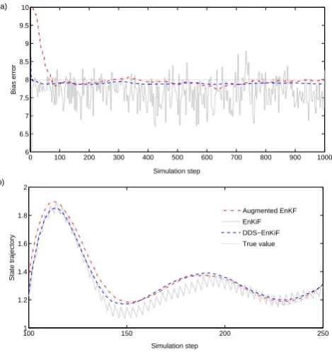
Figure 1 compares the estimation results for 20 ensem-ble members and Q=10−5I,R=10−3I.Part (a) of the figure shows the estimated values of F.The variance of the esti-mates obtained with the EnKiF is clearly much higher than for the other two methods. Incorporating prior knowledge thus significantly reduces the variance of the bias estimate. Note the rather slow convergence of the augmented EnKF compared to the DDS-EnKiF where convergence is almost immediate. Part (b) of the figure shows the estimated values of the system state. Note that the high variance of the bias estimates obtained with the EnKiF has no detrimental effect on the estimated state trajectory.
Table 1 compares the mean square error (MSE) of the es-timatedF-values as function of the measurement noise vari-ance and the varivari-ance of the stochastic model error. The val-ues shown in the table were obtained by averaging the MSE over 1000 consecutive steps, after a converging time of 1000 steps. Results are shown for 20 ensemble members. The model error estimates are more accurate when R decreases. The MSE of the model error estimates also decreases with
Q. However, if Q is very small, the estimates degrade due to
0 200 400 600 800 1000 1200 1400 1600 1800 2000 2
4 6 8 10 12 14
Simulation step
Bias error
0 100 200 300 400 500 600 700 800 900 1000 −6
−4 −2 0 2 4 6 8 10
Simulation step
State trajectory
Augmented EnKF EnKiF DDS−EnKiF True value
(a)
(b)
Fig. 1. Comparison between the assimilation results of an
aug-mented EnKF, the EnKiF and the DDS-EnKiF for the example deal-ing with constant bias errors. (a) The variance of the bias estimates obtained with the EnKiF is much higher than for the other two meth-ods. (b) However, this has no detrimental effect on the estimated state trajectory. Results are shown for 20 ensemble members and
Q=10−5I,R=10−3I.
Table 1. Comparison between the mean square error of the
esti-matedF−values obtained with the EnKiF and the DDS-EnKiF as
function of the measurement noise variance R and the variance of the stochastic model error Q. Results are shown for 20 ensemble members.
Q R
10−2I 10−4I 10−6I 10−8I
10−2I DDS-EnKiF 2.10−2 7.10−3 9.10−3 7.10−3
EnKiF 45 30 31 31
10−4I DDS-EnKiF 4.10−3 8.10−4 1.10−3 7.10−4
EnKiF 26 4.10−1 3.10−1 3.10−1
10−6I DDS-EnKiF 1.10−2 4.10−3 7.10−4 7.10−4
EnKiF 23 3.10−2 7.10−3 6.10−3
10−8I DDS-EnKiF 2.10−1 6.10−3 3.10−3 7.10−4
EnKiF 45 7.10−1 3.10−2 3.10−3
the high variance of the model error estimates obtained with the EnKiF has no detrimental effect on the state estimates.
In real-life data assimilation applications, measurements may not be available at every assimilation time. Figure 2 ex-plores what happens when the time between measurements
0 100 200 300 400 500 600 700 800 900 1000 6
6.5 7 7.5 8 8.5 9 9.5 10
Simulation step
Bias error
1001 150 200 250
1.2 1.4 1.6 1.8 2
Simulation step
State trajectory
Augmented EnKF EnKiF DDS−EnKiF True value
(a)
(b)
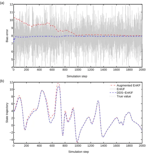
Fig. 2. Comparison between the model error estimates (a) and the
state estimates (b) of the augmented EnKF, the EnKiF and the
DDS-EnKiF when the time between measurements equals 31t.Results
are shown for Q=10−6I,R=10−4I and 20 ensemble members.
equals 31t.The second and the third step of the EnKiF can then be applied at only one out of three assimilation times. The estimatesdˆak−1obtained with the EnKiF thus represent the build-up of the systematic model error over three steps. Part (a) of Fig. 2 compares the estimated values of the model error obtained with the augmented EnKF, the DDS-EnKiF and the EnKiF. The estimates of the EnKiF shown in the fig-ure are obtained by dividingdˆak−1by three. Part (b) of Fig. 2 shows the estimated values of the system state. Due to the bias error which is not accounted for in the EnKiF, the state estimate diverges from the true value during two consecutive steps and then re-converges when measurements are assim-ilated. This leads to the behavior seen in Fig. 2. The non-availability of measurements at all assimilation times has mi-nor effect on the augmented EnKF and the DDS-EnKiF, but is detrimental for the accuracy of the EnKiF.
The effect of systematic measurement error and incom-plete measurements is investigated in Fig. 3. This fig-ure shows results for 10 ensemble members, Q=10−6I and
0 200 400 600 800 1000 1200 1400 1600 1800 2000 4
5 6 7 8 9 10 11 12
Simulation step
Bias error
Kitanidis EnKF Augmented EnKF EnKiF Real
0 200 400 600 800 1000 1200 1400 1600 1800 2000 −4
−2 0 2 4 6 8 10 12
Simulation step
State trajectory
Augmented EnKF EnKiF DDS−EnKiF True value
(a)
(b)
Fig. 3. Effect of systematic measurement error and incomplete
mea-surements on the estimation accuracy. (a) Comparison between the bias estimates obtained with an augmented EnKF, the EnKiF
and the DDS-EnKiF. (b) Estimated trajectory of state variablex20,
which is not measured. Results are shown for Q=10−6I, R=10−4I
and 10 ensemble members.
DDS-EnKiF increases from 8.10−3in case of unbiased mea-surements to 1,1.10−2 in case of systematic measurement error. The systematic measurement error has thus only small detrimental effect on the accuracy of the state estimates.
Now, consider the case where the model is subject to a time-varying bias error of which the dynamics are not known, such that the DDS-EnKiF and the augmented EnKF can not be used. Figure 4 shows the true value of the bias error and the estimate obtained with the EnKiF for
Q=10−6I,R=10−4I and 20 ensemble members. Like in the
example dealing with constant bias errors, the estimates ob-tained with the EnKiF are rather noisy. However, the EnKiF is able to follow the fast variations in the bias error.
6.2 Non-smooth disturbances
In a second example, the true states of the system are taken as the trajectories of the one-level Lorenz model (withN=40 and F=8) obtained with the Runge-Kutta scheme, where Gaussian white process noise with variance Q=10−2I is
added to the discretized state variables and where a non-smooth disturbance is added to state variablex21 at time in-stant 5001t. This disturbance has a peak value of 5 and a duration of 101t. We compare the assimilation results ob-tained with the EnKF, where the disturbance is neglected, to
0 100 200 300 400 500 600 700 800 900 1000 3
4 5 6 7 8 9 10 11 12 13
Simulation step
Bias error
EnKiF True value
Fig. 4. Model error estimates obtained with the EnKiF for the
ex-ample dealing with time-varying bias errors. Like in the exex-ample dealing with constant bias errors, the estimates obtained with the EnKiF are rather noisy. However, the EnKiF is able to follow the
fast variations in the bias errors. Results are shown for Q=10−6I,
R=10−4I and 20 ensemble members.
the results of the EnKiF. Results are presented for 20 ensem-ble members and it is assumed that noisy measurements of all state variables, exceptx20,are available. The measure-ment noise is Gaussian white with variance R=10−3I. Fig-ure 5a shows the true trajectory of state variablex21and the trajectory that would be obtained if no disturbance would be present. The estimates of the EnKF and the EnKiF are also shown. The EnKF looses the true trajectory at the time the disturbances strikes, but quickly re-converges when the dis-turbance has disappeared. The performance of the EnKiF is better, it almost performs as if no disturbance is present. Fig-ure 5b shows the trajectories for state variablex20 which is not affected by a disturbance, but not measured either. The same conclusions apply here.
6.3 Errors due to unresolved scales
495 500 505 510 515 520 525 530 −5
0 5 10 15 20
Simulation step
x21
495 500 505 510 515 520 525 530 −10
−5 0 5 10 15
Simulation step
x20
EnKF EnKiF True value Disturbance−free evolution of true state EnKF EnKiF True value Disturbance−free evolution of true state
(a)
(b)
Fig. 5. Comparison between the assimilation results of the EnKF
and the EnKiF for the Lorenz model subject to a high non-smooth
disturbance. Results are shown for 20 ensemble members and
Q=10−2I, R=10−3I.(a) Results for state variablex21,which is
measured, but affected by a disturbance. (b) Results for state
vari-ablex20,which is not affected by a disturbance, but not measured
either.
constant forcing term is adopted to model the influence of un-resolved fine-scale variables on the large-scale variables. The stochastic model error is assumed to be Gaussian white with variance Qx=10−6I for the discretized large-scale variable and variance Qy=10−8I for the discretized small-scale vari-able. It is assumed that noisy measurements of all large-scale variables are available. The measurement noise is Gaussian white with R=10−6I.For these choices, the error in the mea-surements is approximately ten times smaller than the mag-nitude of the error due to unresolved scales.
The aim of this experiment is twofold. Firstly, we want to obtain an accurate estimate of the model error affecting state variablesx15, x16 andx17.Secondly, we want to ac-count for the model error affecting all other state variables by using an extension of the additive error approach devel-oped by Mitchell and Houtekamer (2002) and used by Hamill and Whitaker (2005) to account for errors due to unresolved scales. In this approach, systematic model errors are ac-counted for by treating them like random white noise with artificially chosen variance. The aim of this experiment is to design a procedure in which this variance is computed from the estimates of the filter.
2500 3000 3500 4000 4500 5000 −0.1
−0.05 0 0.05 0.1
Simulation step
Model error
EnKiF "True" value
2500 3000 3500 4000 4500 5000 −0.05
−0.04 −0.03 −0.02 −0.01 0 0.01 0.02 0.03 0.04 0.05
Simulation step
Model error
First run: Q = 10−6 In
Second run: Q = 3,3.10−4 In
EnKiF "True" value
(a)
(b)
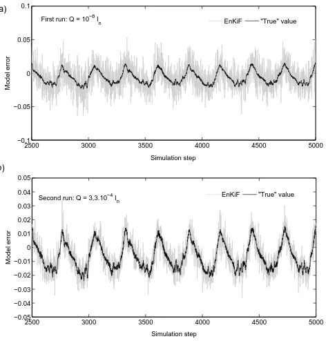
Fig. 6. True and estimated value of the error due to unresolved
scales affecting state variablex16. The model is taken to be the
one-level Lorenz model, while measurements are generated using
the two-level Lorenz model. (a) Results for Q=10−6I.(b) Results
for Q=3,3.10−4I.
In order for the EnKiF to yield estimates of the model error affecting state variablesx15 tox17,we choose the G-matrix as G=[03×14I303×15]T.The value of Q in the EnKiF is cho-sen to be Q=10−6I,which is the variance of the stochastic model error affecting the large-scale variable in the true sys-tem. In the second step of the EnKiF algorithm, we apply covariance localization such that the model error affecting state variablesx15 tox17 is estimated from innovations de-pending on estimates of state variablesx15 tox17 only. All other innovations are inappropriate for estimating the model error affectingx15 tox17 due to the fact that these innova-tions depend on state estimates which are not accounted for model error. The true and estimated value of the model er-ror affecting the state variable with index 16,are shown in Fig. 6a. The true value of the model error at time instantk, is computed by
dk =Ftlk−1(x tl k−1)−F
ol k−1(T(x
tl
k−1)), (55) where Ftlk−1(·) is the two-level Lorenz model operator,
Folk−1(·)is the one-level Lorenz model operator and where
T(·)projects the state of the two-level model to the one-level model.
whereσ2 is the variance of the errors. We approximateσ by computing the standard deviation of the estimated model error affectingx16 over 5000 consecutive steps. The com-puted standard deviation equalss1=0,018. Next, we apply the EnKiF with Q=10−6I for state variablesx15 tox17, but with Q=s12I for all other state variables. The true and
esti-mated value of the model error affecting x16 are shown in Fig. 6b. Estimation accuracy has clearly increased. This improvement is also noticeable in the MSE of the state es-timates, which has dropped from 1,3.10−3in the first run to 3,6.10−4in this run. The standard deviation of the estimated model error affectingx16now equalss2=0,011.
In a third step, we repeat the same procedure, with
Q=10−6I for state variablesx15 tox17 and with Q=s2 2I for all other state variables. The standard deviation of the model error affectingx16 now equals s3=0,012.This values lies close tos2,which indicates that shas almost converged to the optimal value which lies around 0,012.Table 2 summa-rizes the results obtained in the three steps.
The method described above can be used to tune the vari-ance of the random numbers in the additive error approach of Mitchell and Houtekamer (2002). In real-life applications, where the dimension of the measurement vector is much smaller than the dimension of the state vector, the matrix Gk can for example be chosen to estimate the errors affecting a limited number of state variables of which the value is incor-porated into the measurements. For such a choice of Gk,the rank condition (27) is always satisfied. The method described above can then be used to obtain an estimate of the errors af-fecting these state variables. Based on these estimates of the model error, the variance of the random numbers to be used in the approach of Mitchell and Houtekamer (2002) can be tuned.
7 Conclusion and discussion
A new methodology was developed to estimate and account for additive systematic model error in linear filtering as well as in nonlinear ensemble based data assimilation. In contrast to existing methodologies, the approach adopted in this paper can also deal with the case where no dynamical model for the error is available.
In case no model for the error is available, the filter is re-ferred to as EnKiF. The applicability of the EnKiF is limited by the available computational power and by a matrix rank condition which has to be satisfied in order for the filter to exist. The EnKiF can therefore not be used to correct the entire state vector for all possible types of systematic errors. The intended use is therefore to obtain, possibly for a limited number of state variables, an idea about the additive effect of the model error affecting these state variables. This is espe-cially useful if the dynamics of the error are unknown, e.g. in case of unknown time-varying bias errors or errors due to unresolved scales. The estimates of the model error might
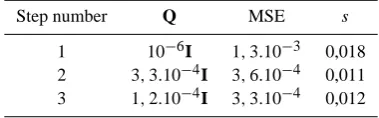
Table 2. Results obtained in the three consecutive experiments
deal-ing with errors due to unresolved scales. The matrix Q denotes the variance of the random vectors which are added to the forecasted ensemble members to account for the model error. The column “MSE” shows the mean square error of the state estimates. The last column shows the standard deviation of the estimates of the model
error affectingx16, which is used to compute the Q-matrix of the
next step.
Step number Q MSE s
1 10−6I 1,3.10−3 0,018
2 3,3.10−4I 3,6.10−4 0,011
3 1,2.10−4I 3,3.10−4 0,012
give insight into the dynamics of the error, which might lead to a refinement of the simulation model or might lead to the development of a “model error model” which can then be incorporated into the assimilation procedure.
In case a model for the error is available, the filter is re-ferred to as DDS-EnKiF. It was shown that there is strong connection between the DDS-EnKiF and the efficient sub-optimal filter developed by Dee and Todling (2000). More precisely, our results extend the latter work to time-varying bias errors.
Simulation results on the chaotic Lorenz (1996) model in-dicate that the model error estimates obtained with the EnKiF have a rather high variance. Estimation accuracy is mainly determined by the variances of the measurement error and the stochastic model error. It was shown that the availability of an accurate dynamical model for the error in the DDS-EnKiF strongly reduces the variance of the model error esti-mates. However, results also indicate that the high variance of the model error estimates obtained with the EnKiF has only minor detrimental effect on the state estimates.
Furthermore, simulation results indicate that the EnKiF and DDS-EnKiF are robust against systematic errors in the measurements. The non-availability of measurements at all assimilation times is detrimental for the accuracy of the EnKiF, but has only minor effect on the DDS-EnKiF be-cause of the error model. The example dealing with constant bias errors indicates that both methods behave similarly as the number of measurements in space decreases.
Appendix A
Calculation of optimal gain matrix
In this Appendix, we prove the optimality of the filter (32)– (38) for the case where conditions (29)–(30) are satisfied. We show that under the latter conditions the gain matrix (37) minimizes the variance of (36).
Using (32)–(38), we find that
Pak =KxkR¯¯kKxkT−K x
kS¯¯k−S¯¯TkK xT
k +P a∗
k , (A1)
where
¯¯
Rk =CkPka∗CTk +Rk−EkKdkRk−RkKdkTETk, (A2)
¯¯
Sk =CkPak∗−RkKdkTGTk−1, (A3)
Pak∗=E[(xk−xˆka∗)(xk−xˆak∗)T], (A4)
=(I−Gk−1KdkCk)(Pkf+Gk−1Pkf,d−1GTk−1)
(I−Gk−1KdkCk)T+Gk−1KdkRkKdkTGTk−1. (A5) Note that these equations are valid only if conditions (29)– (30) are satisfied. The gain matrix Kxk minimizing the trace of (A1), is given by
Kxk =S¯¯TkR¯¯−k1. (A6)
Finally, substituting (A2) and (A3) in (A6), yields after a straightforward calculation
Kxk =PfkCTk(CkPfkCTk +Rk)−1. (A7)
Appendix B
Proof of convergence
In this Appendix, we give an outline of the proof that, in case of a linear model operator, the EnKiF converges to the filter developed by Gillijns and De Moor (2007) forq→∞.Using the fact that the EnKF converges to the Kalman filter in case of a linear model, we only need to show that Eqs. (48)–(50) converge to the corresponding equations in Sect. 3.2. This basically comes down to showing that the sample variance of δki−1converges to (26). This sample variance is given by
1 q−1
q
X
i=1
¯
δk−1−δki−1 δ¯k−1−δki−1
T
= ¯MkR¯kM¯Tk.
(B1) It follows from the convergence of the EnKF to the Kalman filter thatR¯kconverges toR˜k forq→∞.Consequently (B1) converges to (26). If no perturbed observations are used in (49), the sample variance would converge to MkCkPfkCTkMTk and would thus underestimate (26).
Appendix C
The Lorenz (1996) model
The equations for the one-level Lorenz (1996) model are given by
dxi
dt =(xi+1−xi−2)xi−1−xi +F, (C1) where the index i=1, . . . , N is cyclic so that xi−N=xi+N=xi.
The equations for the two-level model are given by dxi
dt =(xi+1−xi−2)xi−1−xi +F− c b
M
X
j=1
yi,j, (C2) dyi,j
dt =cb(yi,j−1−yi,j+2)yi,j+1−cyi,j + c
bxi, (C3) fori=1, . . . , N andj=1, . . . , M.The indices are cyclic so that for exampleyi,j+M=yi+1,jandyi+N,j=yi,j.
Acknowledgements. Our research is supported by Research Council KULeuven: GOA AMBioRICS, several PhD/postdoc & fellow grants; Flemish Government: FWO: PhD/postdoc grants, projects, G.0407.02 (support vector machines), G.0197.02 (power islands), G.0141.03 (Identification and cryptography), G.0491.03 (control for intensive care glycemia), G.0120.03 (QIT), G.0452.04 (new quantum algorithms), G.0499.04 (Statistics), G.0211.05 (Nonlinear), research communities (ICCoS, ANMMM, MLDM); IWT: PhD Grants, GBOU (McKnow); Belgian Federal Science Policy Office: IUAP P5/22 (‘Dynamical Systems and Control: Computation, Identification and Modelling’, 2002-2006); PODO-II (CP/40: TMS and Sustainability); EU: FP5-Quprodis; ERNSI; Contract Research/agreements: ISMC/IPCOS, Data4s, TML, Elia, LMS, Mastercard.
Edited by: O. Talagrand Reviewed by: two referees
References
Anderson, J.: An ensemble adjustment Kalman filter for data as-similation, Mon. Wea. Rev., 129, 2884–2903, 2001.
Anderson, J. and Anderson, S.: A Monte Carlo implementation of the nonlinear filtering problem to produce ensemble assimi-lations and forecasts, Mon. Wea. Rev., 127, 2741–2758, 1999. Bishop, C., Etherton, B., and Majundar, S.: Adaptive sampling with
the ensemble transform Kalman filter. Part I: theoretical aspects, Mon. Wea. Rev., 129, 420–436, 2001.
Burgers, G., van Leeuwen, P., and Evensen, G.: Analysis scheme in the ensemble Kalman filter, Mon. Wea. Rev., 126, 1719–1724, 1998.
Dee, D. and Da Silva, A.: Data assimilation in the presence of fore-cast bias, Quart. J. Roy. Meteorol. Soc., 117, 269–295, 1998. Dee, D. and Todling, R.: Data assimilation in the presence of
Evensen, G.: Sequential data assimilation with a nonlinear quasi-geostrophic model using Monte Carlo methods to forecast error statistics, J. Geophys. Res., 99, 10 143–10 162, 1994.
Evensen, G.: The ensemble Kalman filter: theoretical formulation and practical implementation, Ocean Dyn., 53, 343–367, 2003. Friedland, B.: Treatment of bias in recursive filtering, IEEE Trans.
Autom. Control, 14, 359–367, 1969.
Gillijns, S. and De Moor, B.: Unbiased minimum-variance input and state estimation for linear discrete-time systems, Automat-ica, 43, 111–116, 2007.
Griffith, A. and Nichols, N.: Adjoint methods in data assimilation for estimating model error, J. Flow Turbulence Combust., 65, 469–488, 2000.
Hamill, T. and Whitaker, J.: Accounting for the error due to un-resolved scales in ensemble data assimilation: a comparison of different approaches, Mon. Wea. Rev., 133, 3132–3147, 2005. Hamill, T., Whitaker, J., and Snyder, C.: Distance-dependent
fil-tering of background-error covariance estimates in an ensemble Kalman filter, Mon. Wea. Rev., 129, 2776–2790, 2001.
Heemink, A., Verlaan, M., and Segers, A.: Variance reduced ensem-ble Kalman filtering, Mon. Wea. Rev., 129, 1718–1728, 2001. Houtekamer, P. and Mitchell, H.: A sequential ensemble Kalman
filter for atmospheric data assimilation, Mon. Wea. Rev., 129, 123–137, 2001.
Kailath, T., Sayed, A., and Hassibi, B.: Linear Estimation, Prentice Hall, Upper Saddle River, New Jersey, 2000.
Kitanidis, P.: Unbiased minimum-variance linear state estimation, Automatica, 23, 775–778, 1987.
Lorenz, E.: Predictability: A problem partly solved, in: Proc. ECMWF Seminar on Predictability, Vol. I, pp. 1–18, 1996.
Martin, M., Bell, M., and Nichols, K.: Estimation of systematic error in an equatorial ocean model using data assimilation, Int. J. Numer. Fluids, 40, 435–444, 2002.
Mitchell, H. and Houtekamer, P.: Ensemble size, balance, and model-error representation in an ensemble Kalman filter, Mon. Wea. Rev., 130, 2791–2808, 2002.
Orrell, D., Smith, L., Barkmeijer, J., and Palmer, T.: Model error in weather forecasting, Nonlin. Processes Geophys., 8, 357–371, 2001,
http://www.nonlin-processes-geophys.net/8/357/2001/.
Ott, E., Hunt, B., Szunyogh, I., Zimin, A., Kostelich, E., Corazza, M., Kalnay, E., Patil, D., and Yorke, J.: A local ensemble Kalman filter for atmospheric data assimilation, Tellus, 56A, 415–428, 2002.
Reichle, R., McLaughlin, D., and Entekhabi, D.: Hydrologic data assimilation with the ensemble Kalman filter, Mon. Wea. Rev., 130, 103–114, 2002.
Tippett, M., Anderson, J., Bishop, C., Hamill, T., and Whitaker, J.: Ensemble square root filters, Mon. Wea. Rev., 131, 1485–1490, 2003.
Whitaker, J. and Hamill, T.: Ensemble data assimilation without perturbed observations, Mon. Wea. Rev., 130, 1913–1924, 2002. Zupanski, D.: A general weak constraint applicable to operational 4DVAR data assimilation systems, Mon. Wea. Rev., 125, 2274– 2292, 1997.