www.atmos-meas-tech.net/9/2043/2016/ doi:10.5194/amt-9-2043-2016
© Author(s) 2016. CC Attribution 3.0 License.
Approaches to radar reflectivity bias correction to improve
rainfall estimation in Korea
Cheol-Hwan You1, Mi-Young Kang2, Dong-In Lee1,2, and Jung-Tae Lee2
1Atmospheric Environmental Research Institute, Pukyong National University, Busan, South Korea 2Department of Environmental Atmospheric Sciences, Pukyong National University, Busan, South Korea
Correspondence to: Dong-In Lee ([email protected])
Received: 13 December 2015 – Published in Atmos. Meas. Tech. Discuss.: 18 January 2016 Revised: 6 April 2016 – Accepted: 22 April 2016 – Published: 4 May 2016
Abstract. Three methods for determining the reflectivity bias of single polarization radar using dual polarization radar re-flectivity and disdrometer data (i.e., the equidistance line, overlapping area, and disdrometer methods) are proposed and evaluated for two low-pressure rainfall events that oc-curred over the Korean Peninsula on 25 August 2014 and 8 September 2012. Single polarization radar reflectivity was underestimated by more than 12 and 7 dB in the two rain events, respectively. All methods improved the accuracy of rainfall estimation, except for one case where drop size dis-tributions were not observed, as the precipitation system did not pass through the disdrometer location. The use of these bias correction methods reduced the RMSE by as much as 50 %. Overall, the most accurate rainfall estimates were ob-tained using the overlapping area method to correct radar re-flectivity.
1 Introduction
Radar is a useful remote sensing instrument for measuring rainfall amount due to its relatively high resolution in both space and time. Areal rainfall rate must be derived from radar reflectivity, not measured directly. This estimation of radar rainfall is based on the relationship between reflectivity (Z) and rainfall rate (R), known as theZ−Rrelation (R(Z)). Ex-perimentally measured drop size distributions (DSDs) have been used extensively to obtain both radar reflectivity and rainfall rate (Compos and Zawadzki, 2000; Jang et al., 2004; You et al., 2004). There is no uniqueR(Z), since DSDs can be varied storm to storm and even within a single storm (Bat-tan, 1973; You et al., 2010).
However, radar rainfall estimation is complicated by a number of uncertainties including hardware calibration, par-tial beam filling, rain attenuation, bright band, and non-weather echoes (Wilson and Brandes, 1979; Austin, 1987). The correction of bias in Z caused by hardware calibra-tion error is difficult to achieve using single polarimetric radar (SPOL) alone. Polarimetric radar (DPOL) provides a new method for the absolute calibration of reflectivity, which has been a longstanding problem with single polarization radar data. The method is based on the assumptions thatZ, differential reflectivity (ZDR), and specific differential phase (KDP)are independent of each other and thatZ can be es-timated fromZDRandKDP, which are insensitive to radar miscalibration (Gorgucci et al., 1992, 1999; Goddard et al., 1994; Scarchilli et al., 1996; Vivekanandan et al., 1999).
The Korea Meteorological Administration (KMA) is in the process of replacing Doppler radars with S-band DPOLs (to be completed by 2019), and the Ministry of Land, Infras-tructure, and Transport (MoLIT) has installed four S-band DPOLs for operational use since 2009. Until the DPOL in-stallation is complete, it is necessary to use a combination of SPOLs and DPOLs to produce rainfall mosaics covering the whole Korean Peninsula. To obtain more accurate mo-saicked radar rainfall, SPOL reflectivity should be corrected using the reflectivity of DPOLs and other instruments such as the disdrometer. Accurate SPOL reflectivity is also required for climatological analysis using radar rainfall.
re-BSL PSN AWS
60 km 120 km
180 km 240 km
Longitude (East)
Latitude (North)
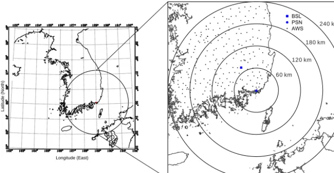
Figure 1. Location of the Bislsan radar (solid rectangle), the PARSIVEL disdrometer and Gudeok radar (solid circle), and rain gages (black
dots) distributed within 240 km of radar coverage. Circles indicate distance from the Gudeok radar and are drawn at intervals of 60 km.
flectivity andZDRand for validation. In Sect. 3, the results obtained using the three correction methods are compared with gage measurements. Finally, we summarize the results and provide conclusions in Sect. 4.
2 Data
Rainfall data from rain gages operated by the KMA were used to evaluate the accuracy of radar rainfall. Rain gages located between 5 and 134 km from the radar were included in the analysis. Figure 1 shows the location of all instruments used in this study. The PARSIVEL (PARticle SIze VELocity) disdrometer was installed∼9 km from PSN (Pusan radar). PARSIVEL is a laser-optic system that measures 32 chan-nels from 0.062 to 24.5 mm (for detailed specifications, see Loffler-Mang and Joss, 2000).
Data observed from PARSIVEL were regarded as unreli-able and removed from the analysis in the case that any of the following conditions were met: 1 min rain rate was less than 0.1 mm h−1; total number concentration from all channels was less than 10; drop numbers were recorded only in the lower 10 channels (1.187 mm for PARSIVEL); drop num-bers were recorded only in the lower 5 channels (0.562 mm for PARSIVEL) (You and Lee, 2015).
Radar data were recorded at PSN (Pusan radar), which is located at the coastal line, and BSL (Bislsan radar), which is located 76.9 km away from PSN (Fig. 1); these radars were installed and are operated by KMA and MoLIT, respectively. The transmitted peak power of BSL is 750 kW, the beam width is 0.95◦, the frequency is 2.791 GHz, and the antenna is 1085 m above sea level (m a.s.l.). The polarimetric vari-ables are estimated with a gate size of 0.125 km. The scan strategy consists of six elevation angles with a 2.5 min update interval. The transmitted peak power of PSN is 800 kW, the beam width is 1.0◦, the frequency is 2.712 GHz, and the
an-Table 1. Rainfall events used for the analysis.
Date Source Period of analysis
8 September 2012 Low pressure 00:00 to 06:00 LST 25 August 2014 Low pressure 09:00 to 16:00 LST
tenna is 547 m a.s.l. The reflectivity is estimated with a gate size of 0.25 km. The PSN scan strategy consists of 13 ele-vation angles with a 10 min update interval. Radar variables at an elevation angle of 0.5 (1.8)◦were extracted from the
BSL (PSN) data every 10 min, to match the time interval for this study. Non-meteorological targets were removed from the PSN data using the texture and vertical gradient of reflec-tivity, as proposed by Zhang et al. (2004). Polarimetric vari-ables were subjected to quality control using a threshold of 15◦for the standard deviation of the differential phase shift (You et al., 2014).
The quality controlledZH,ZDR, andKDPmeasured from BSL were used to calibrateZDR andZH of BSL. The ZH measured from PSN was then corrected by using calibrated ZHof BSL using self-consistency method andZHmeasured by PARSIVEL. The gage rainfall data were used to assess the performance of threeZH bias correction methods for PSN which is SPOL.
The accuracy of rainfall estimation using corrected reflec-tivity was evaluated to measure the effectiveness of each method for calculating the difference reflectivity between PSN and BSL (PARSIVEL). Two rainfall events were used, occurring on 25 August 2014 and 8 September 2012 (Ta-ble 1). The August and September events were caused by low-pressure systems over the Korean Peninsula, respec-tively.
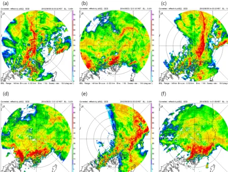
pre-Figure 2. Time series of horizontal reflectivity (ZH) at 0.5 elevation angle observed from BSL (a) 04:00 LT, (c) 05:00 LT, and (e) 06:00 LT on 8 September 2012 and (b) 12:00 LT, (d) 13:00 LT, and (f) 14:00 LT on 25 August 2014.
cipitation within radar coverage on 8 September 2012 was caused by low pressure with the front located at northern part of Korea. The core of the precipitation systems elongated from south to north and moved eastward. The maximum reflectivity of the core was more than 45 dBZ and caused rainfall in the western part of radar coverage at 03:00 LST (Fig. 2a), became more organized at the eastern part of radar coverage at 04:00 LST (Fig. 2c), and moved eastward and were located around the coast at 05:00 LST (Fig. 2e) on 8 September 2012. The precipitation system on 25 August 2014 was caused by the low pressure located in the south-ern part of Korea. The two areas of strong rainfall within the radar coverage were located in the southwestern part of the radar coverage with distance between 120 and 150 km and in the southern part of the radar coverage with distance between 30 and 90 km at 12:00 LST on 25 August 2014 (Fig. 2b). The two convective cells moved eastward, their strength intensi-fied, and the area of rainfall was wider at 13:00 LST (Fig. 2d). The two systems moved eastward continuously and merged together at 14:00 LST (Fig. 2f).
Figure 3 shows the time series of hourly rainfall and daily accumulation measured by a gage which recorded highest daily rainfall within radar coverage on 8 September 2012 and 25 August 2014. The highest daily accumulated rainfall was recorded from North Changwon (ID 255) and Geum-jeong (ID 939) on each day, respectively. The daily accu-mulation of ID 255 was 150 mm, the maximum hourly rain-fall was around 40 mm, and the duration of the rainrain-fall was 7 h (Fig. 3a). The daily accumulation of ID 939 was around 270 mm and the maximum hourly rainfall was more than 100 mm h−1. The rainfall amount for 3 h (10:00, 14:00, and 15:00 LST) mainly contributed to the total rainfall accumu-lation on 25 August 2014 (Fig. 3b).
3 Methodology
3.1 ZandZDRbias correction for BSL
(a)
(b)
Hourly rainfall (mm)
Hourly rainfall (mm) Accumulation (mm)
Accumulation (mm)
Time (h, LST)
Time (h, LST)
Figure 3. Time series of 1 h rainfall (bar) and daily accumulated
(red line) measured from a gage which recorded highest daily rain-fall within radar coverage at (a) North Changwon (ID 255) on 8 September 2012 and (b) Geumjeong (ID 939) on 25 August 2014.
using a vertical pointing scan of light rain to take advan-tage of the nearly spherical shape of the raindrops as seen from below. Ryzhkov et al. (2005) used the elevation an-gle dependency ofZDRas an alternative technique and con-cluded that the high variability ofZDRin rainfall prohibited the method from achieving the required absolute calibration accuracy of 0.2 dB. They instead proposed a method that utilizes the structural characteristics of the melting layer in stratiform clouds and the dry aggregated snow present above the melting layer. ZDR measurements from dry aggregated snow above the melting layer resulted in a mean S-band value of 0.2 dB and an accuracy of 0.1–0.2 dB. Trabal et al. (2009) evaluated two methods using the intrinsic properties of dry aggregated snow present above the melting layer and light rain measurements close to the ground and found that aZDR calibration accuracy of 0.2 dB or better was achieved using either method.
Vertical pointing data were not available in the present case, and the scan strategy, with six elevation angles, was unable to detect the melting layer. Therefore, in this study, light rain measurements close to the ground were used to calibrate ZDR. Light rain was defined using a threshold of 20 dBZ≤Z≤28 dBZ, as proposed by Marks et al. (2011). The assumption ofZDRis close to 0 in the case of the small raindrop-like drizzle chosen for this study. TheZDRvalues observed from BSL with reflectivity in the range of 20 to
28 dBZ for a given time period were averaged. Then the av-eragedZDRwas taken as aZDRbias.
TheZH bias was calculated by a self-consistency method using a nine-gate moving average of bias-correctedZDRin the range of 0.2 to 3.0 dB to improve the accuracy. This method depends on the notion thatZH,ZDR, andKDP are independent in rain and thatZHcan be estimated fromZDR andKDP. The difference between the computed and observed values of ZH is referred to as the Z bias. Following the method of Ryzhkov et al. (2005), the entire spatial and tem-poral domain was divided into 1 dB intervals ofZHbetween Zmin (30 dBZ) and Zmax (50 dBZ), and theKDP (ZH) and ZDR(ZH)within each interval were calculated. TheZHbias is then determined by matching the integrals as follows: I1=
Zmax
X
Zmin
KDP(Z)n(Z)1Z, (1)
I2=
Zmax
X
Zmin
100.1Zmf (Z
DR)n(Z)1Z, (2)
The function off (ZDR)in Eq. (2) can be well approximated by a fourth-order polynomial fit for certain range of ZDR (Gourley et al., 2009) like Eq. (3).
f (ZDR)=10−5(a0+a1ZDR+a2Z2DR+a3ZDR3 ). (3) The estimatedZH bias is determined from Vivekanandan et al. (2003) by
ZHbias(dB)=10 log( I2 I1
), (4)
If the radar is well calibrated,ZH bias should be equal to 0. The coefficients off (ZDR)were calculated byT-matrix scattering method using long period DSD data and are 4.26,
−4.67, 2.67, and−0.54, respectively. 3.2 Equidistance line method
To calculate the reflectivity bias of PSN, which is a single po-larization radar, three approaches were used: the equidistance line method, the overlapping area method, and the disdrome-ter method. The first approach is to compare the reflectivities along the line that is equidistant between the two radars. To determine this line for the two radars, the effective radius was set to 100 km, and the distance between the two radars and the azimuthal angle pointing from BSL to PSN were calcu-lated using their latitude and longitude values. The start and end azimuthal angles for comparison of reflectivity were then calculated as follows:
AZst=β−acos(0.5×dr/rc), (5)
which is the angle between north and the bearing from BSL points to PSN and rc and dr are the effective radius and dis-tance from BSL to PSN, respectively. The disdis-tance between the two radars is 76.9 km, and the start and end azimuthal an-gles of BSL (PSN) are 79 (35) and 213 (261)◦, respectively (Fig. 4).
To compare the reflectivity observed of targets at the al-most same height from both radars, the beam height was cal-culated assuming a standard atmospheric beam propagation (Rinehart, 2010), as follows:
H=
q
r2+(R0+H
0)2+2r(R0+H0)sinϕ−R0, (7) whereris the slant range from the radar,ϕis the elevation angle of the radar beam,H0is the height of the radar antenna above sea level, andR0=(4/3)R, whereRis the Earth’s ra-dius (6371 km). The radar antenna heights of PSN and BSL are 547 and 1085 m, respectively. Figure 5 shows the beam height of PSN with blue solid line and BSL at the equidis-tance line (blue dashed line as shown in Fig. 4). EL1 to EL6 show the elevation angles from smallest to largest. The smallest difference in beam height between the two radars is 149 m, which was obtained using the fourth elevation an-gle of PSN and the third elevation anan-gle of BSL. Therefore, the reflectivity bias of PSN was calculated by averaging the difference of reflectivity along with the equidistance line ob-served from the fourth elevation angle of PSN and the third one of BSL.
3.3 Overlapping area method
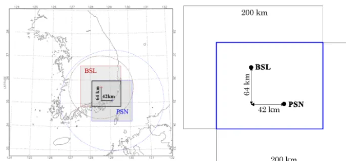
In the second approach, the overlapping area for the two radars was calculated by matching the coordinates. The polar coordinate of two radars was converted to a Cartesian coordi-nate with a spatial resolution of 1 km. The overlapping area was then determined by considering the distances between the two radars in the east–west and north–south directions. Figure 6 shows a schematic diagram of the overlapping area for the two radars. The distance between the two radars in east–west and north–south direction is 42 and 64 km, respec-tively. The reflectivity observed from both radars at the pixels designated at the overlapping area as shown by a blue rect-angle in the right panel of Fig. 6, was compared to calculate theZHbias of PSN. The extracted domain of PSN and BSL for the comparison is 158×136 km.
3.4 Disdrometer method
The third and final approach is to use DSD observations from the PARSIVEL disdrometer. The reflectivity was cal-culated from the DSD at 1 min resolution and averaged over 10 min to match the radar time resolution. Figure 7 shows a schematic of the procedure used to match the radar and PAR-SIVEL data. The PARPAR-SIVEL disdrometer is located∼9 km from the radar, at an azimuthal angle of 87◦. The radar re-flectivity was averaged over a domain of 13 gates×3◦ in
BSL
PSN
1
0
0
km
76 .9 k
m β=147.6°
Start Azimuth
BSL : 79° PSN : 35°
End Azimuth
BSL : 213° PSN : 261°
Equidistance line
Figure 4. Schematic diagram showing the method used to calculate
the line of equidistance between two radars. The effective radius was set to 100 km and the distance between radars is 76.9 km. The azimuthal angle from BSL to PSN is 147.6◦. The start and end az-imuthal angles are 79 (35) and 213 (261)◦for BSL (PSN), respec-tively. The blue dashed line shows the equidistance line.
0 20 40 60 80 100 120
0 1 2 3 4 5
0 20 40 60 80 100 120
Gate number 0
1 2 3 4 5
Height (km)
PSN BSL
EL1 EL2 EL3 EL4 EL5 EL6
Figure 5. Beam height of PSN (blue solid lines) and BSL (red
dot-ted lines) at the equidistance line. EL1 to EL6 show the first, second, third, fourth, fifth, and sixth elevation angles, respectively.
azimuth, centered at the PARSIVEL location. The reflectiv-ity observed by BSL or PARSIVEL subtracted from that ob-served by PSN was taken as aZHbias and it will be applied to all pixels of PSN coverage.
3.5 Validation
Figure 6. Schematic diagram of the overlapping area for BSL and PSN. The east–west and north–south distances between the two radars
are 42 and 64 km, respectively. The red (blue) dotted circle shows the maximum range of BSL (PSN) and gray shaded area show 200 km by 200 km extracted from each radar coverage in the left panel.
Figure 7. Schematic diagram showing matching of the radar gate
and the PARSIVEL disdrometer. PARSIVEL is located ∼9 km from the radar, at an azimuthal angle of 87◦. The radar reflectivity was averaged over a 3 km×3◦domain centered at the PARSIVEL location.
These quantities are defined as follows:
NE=
1
N N P
i=1
RR, i−RG, i
RG
, (8)
RMSE=
"
1 N
N X
i=1
(RR, i−RG, i)2
#1/2
, (9)
CC=
N P
i=1
(RR, i−RR)(RG, i−RG)
N
P
i=1
(RR, i−RR)2
1/2N
P
i=1
(RG, i−RG)2
1/2
, (10)
whereN is the number of radar rainfall (RR)and gage rain-fall (RG)pairs, andRR andRG are the average hourly rain rates from radar and gages, respectively. These quantities were calculated using total accumulated rainfall amounts for analyzed time period from radar and gage measurements at each point. The radar rainfall value at each point was ob-tained by averaging rainfall over a small area (1 km×1◦) centered on the corresponding rain gage. The radar rain-fall was calculated using the relation Z=200R1.6 and Z=300R1.4.
4 Results
4.1 Equidistance line method
09 10 11 12 13 14 15 16 −15
−12 −9 −6 −3 0 3 6
09 10 11 12 13 14 15 16
h (LST) −15
−12 −9 −6 −3 0 3 6
Reflectivity difference (dB)
0 20 40 60 80 100 120
Sample number
Average Sample number
Figure 8. Time series of the average reflectivity difference between
PSN and BSL at the equidistance line (blue circles) and the number of samples used in each calculation (black squares) on 25 August 2014.
00 01 02 03 04 05 06
−15 −12 −9 −6 −3 0 3 6
00 01 02 03 04 05 06
h (LST) −15
−12 −9 −6 −3 0 3 6
Reflectivity difference (dB)
0 20 40 60 80 100 120
Sample number
Average Sample number
Figure 9. As for Fig. 8 but for 8 September 2012.
not located enough over the equidistance line to get a reliable comparison until 03:10 LST.
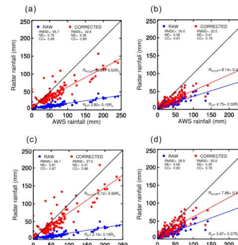
Figure 10 shows the scatter plot of total accumulated radar rainfall amount for the analyzed time period, calculated us-ingZ=200R1.6andZ=300R1.4, and gage rainfall, for 25 August 2014 and 8 September 2012. The RMSE, NE, and CC of rainfall pairs forZ=200R1.6(Z=300R1.4)on 25 Au-gust 2014 were improved from 65.7 (66.1) to 32.6 (27.0) mm, from 0.79 (0.81) to 0.36 (0.31), and from 0.88 (0.87) to 0.89 (0.88), respectively. On 8 September 2012, the RMSE, NE, and CC forZ=200R1.6(Z=300R1.4)changed from 30.0 (28.5) to 22.5 (20.0) mm, from 0.58 (0.56) to 0.41 (0.36), and from 0.81 (0.8) to 0.78 (0.76), respectively, by the use of bias correction. In both cases, the use of corrected reflectivity for rainfall estimation resulted in much better accuracy than us-ing raw reflectivity did.
4.2 Overlapping area method
Figure 11 shows time series of the mean reflectivity differ-ences between PSN and BSL in the overlapping area and the number of samples used for calculation ofZHbias on 25
Au-(a) (b)
(c) (d)
Figure 10. Scatter plot of total accumulated rainfall for
ana-lyzed time period calculated by gage and radar using (a and b)
Z=200R1.6and (c and d)Z=300R1.4for 25 August 2014 and 8 September 2012, respectively. Blue circles show the rainfall pairs obtained using raw reflectivity and red circles show those obtained using reflectivity corrected with the equidistance line method.
09 10 11 12 13 14 15 16
−20 −16 −12 −8 −4 0
09 10 11 12 13 14 15 16
h (LST) −20
−16 −12 −8 −4 0
Reflectivity difference (dB)
0 5000 10 000 15 000 20 000 25 000
Sample number
Average Sample number
Figure 11. Time series of the average reflectivity difference
be-tween PSN and BSL at the overlapping area (blue circles) and the number of samples used in each calculation (black squares) on 25 August 2014.
00 01 02 03 04 05 06 −8
−6 −4 −2 0 2
00 01 02 03 04 05 06
h (LST) −8
−6 −4 −2 0 2
Reflectivity difference (dB)
0 5000 10 000 15 000 20 000 25 000
Sample number
Average Sample number
Figure 12. Time series of the average reflectivity difference
be-tween PSN and BSL at the overlapping area (blue circles) and the number of samples used in each calculation (black squares) on 8 September 2012.
(a) (b)
(c) (d)
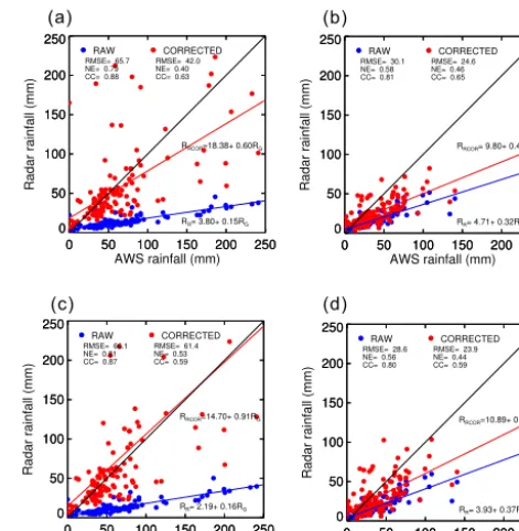
Figure 13. As for Fig. 10 but for the overlapping area method.
corrected by self-consistency. The radar rainfall estimation was done by using observed and correctedZHas an input of Z−Rrelations.
Figure 13 shows a scatter plot of total accumulated radar rainfall amount for the entire analyzed time period, calcu-lated using Z=200R1.6 andZ=300R1.4, and gage rain-fall, for 25 August 2014 and 8 September 2012. The RMSE and NE of rainfall pairs forZ=200R1.6(Z=300R1.4)on 25 August 2014 were improved from 65.7 (66.1) to 29.7 (25.8) mm and from 0.79 (0.81) to 0.31 (0.28), respectively. On 8 September 2012, RMSE and NE for Z=200R1.6 (Z=300R1.4) were improved from 30.0 (28.5) to 21.8 (19.1) mm and from 0.58 (0.56) to 0.40 (0.34), respectively,
00 03 06 09 12 15 18 21 00
0 5 10 15 20 25
00 03 06 09 12 15 18 21 00
h (LST) 0
5 10 15 20 25
Rainfall amount (mm)
AWS PARSIVEL
AWS TOTAL= 116.0 mm PAR TOTAL= 129.4 mm
Figure 14. Time series of 10 min rainfall amount as obtained by
PARSIVEL (red circles) and collocated gages (blue circles).
by the use of bias correction, while CC forZ=200R1.6was unchanged at 0.81 and that ofZ=300R1.4changed from 0.8 to 0.79. Again, in both cases the use of corrected reflectiv-ity for rainfall estimation was found to improve the accuracy compared with raw reflectivity.
4.3 Disdrometer method
Before using the disdrometer bias correction method to esti-mate rainfall rates, 10 min rain rates obtained directly from DSDs and from collocated gages were compared. Figure 14 shows the time series of rain rate obtained by PARSIVEL and collocated gages on 25 August 2014. Daily total rain-fall amounts for PARSIVEL and the gages were 129.4 and 116.0 mm, respectively. The difference in the totals is only 13.4 mm, and the RMSE and CC between the 10 min time se-ries were 0.52 mm h−1and 0.99, respectively. On 8 Septem-ber 2012 (not shown), daily total rainfall amounts for PAR-SIVEL and the gage were 54.4 and 55.0 mm, respectively. The difference between the total daily rainfall amounts was 0.7 mm and the RMSE and CC between the two 10 min se-ries were 0.62 mm h−1and 0.96, respectively. It is concluded that DSDs were sufficiently reliable to use as a reference with which to calculate the radar bias.
re-09 10 11 12 13 14 15 16 −30
−20 −10 0 10 20 30
09 10 11 12 13 14 15 16
h (LST) −30
−20 −10 0 10 20 30
Reflectivity difference (dB)
0 10 20 30 40 50 60
Reflectivity of PARSIVEL (dBZ)
Difference Parsivel
Figure 15. Time series of reflectivity obtained by PARSIVEL (red
circles), and the radar bias (blue circles) on 25 August 2014.
00 01 02 03 04 05 06
−30 −20 −10 0 10 20 30
00 01 02 03 04 05 06
h (LST) −30
−20 −10 0 10 20 30
Reflectivity difference (dB)
0 10 20 30 40 50 60
Reflectivity of PARSIVEL (dBZ)
Difference Parsivel
Figure 16. As for Fig. 15 but for 8 September 2012.
liable only until 12:00 LST. The bias values ranged from
−13.4 to−3.1 dB until 12:00 LST. Figure 16 shows time se-ries of reflectivity obtained by radar and by PARSIVEL and the radar bias on 8 September 2012. On this occasion there were no reflectivity data from either PARSIVEL or radar un-til 03:30 LST. The bias values were distributed from−14.3 to 12.7 dB.
Figure 17 shows a scatter plot of total accumulated radar rainfall amount for the entire time period, calcu-lated using Z=200R1.6 andZ=300R1.4, and gage rain-fall on 25 August 2014 and 8 September 2012. The RMSE and NE of rainfall pairs for Z=200R1.6 (Z=300R1.4) on 25 August 2014 were improved from 65.7 (66.1) mm to 42.0 (61.4) mm and from 0.79 (0.81) to 0.40 (0.53), respectively. On 8 September 2012, RMSE and NE for Z=200R1.6(Z=300R1.4)decreased from 30.1 (28.6) to 24.6 (23.9) mm, and from 0.58 (0.56) to 0.46 (0.44), respec-tively, while CC forZ=200R1.6(Z=300R1.4)decreased from 0.81 (0.8) to 0.65 (0.59). In both cases, using corrected rather than raw reflectivity for rainfall estimation improved accuracy as measured by RMSE and NE but reduced accu-racy as measured by CC.
(a) (b)
(c) (d)
Figure 17. As for Fig. 10 but for the disdrometer method.
4.4 Discussion
(a)
(b) Time (h)
Time (h)
RMSE (mm h )
-1
RMSE (mm h )
-1
Figure 18. Accumulated rainfall RMSE calculated from radar and
gage for different bias correction methods on (a) 25 August 2014 and (b) 8 September 2012. The bars with different colors show re-sults obtained using the raw data (RAW), equidistance line method (LINE), overlapping area method (AREA), and disdrometer method (DSD).
Considering the entire period covering both events, the overlapping area method showed the best performance, as measured by RMSE. The accuracy of radar rainfall estimates could be improved by combining the three approaches, using metrics such as DSD temporal stability and the number of samples available for the equidistance line method to select the best method for a particular situation. It is worth noting that the result would be changed when the drop size distribu-tions was fluctuated with height, especially at the layer be-tween radar beam and ground in the disdrometer method. 4.5 Conclusions
Three methods for determining the reflectivity bias of sin-gle polarization radar using dual polarization radar reflectiv-ity and disdrometer data were proposed and examined for two rainfall events caused by low pressure over the Korean Peninsula on 25 August 2014 and 8 September 2012. Single polarization radar reflectivity was underestimated by more than 12 and 7 dB during the August and September events, respectively. All three methods improved the accuracy of es-timated rainfall, except during a period when DSDs were not
observed (as the precipitation system did not pass over the disdrometer location).
The rainfall estimation using Z=200R1.6 and Z=300R1.4 and gage rainfall were examined for 25 August 2014 and 8 September 2012 to investigate the accuracy of each method. The RMSE, NE, and CC of rainfall pairs forZ=200R1.6(Z=300R1.4)on 25 August 2014 with the equidistance method were improved from 65.7 (66.1) to 32.6 (27.0) mm, from 0.79 (0.81) to 0.36 (0.31), and from 0.88 (0.87) to 0.89 (0.88), respectively. On 8 September 2012, the RMSE, NE, and CC forZ=200R1.6 (Z=300R1.4)changed from 30.0 (28.5) to 22.5 (20.0) mm, from 0.58 (0.56) to 0.41 (0.36), and from 0.81 (0.8) to 0.78 (0.76), respectively.
The RMSE and NE of rainfall pairs for Z=200R1.6 (Z=300R1.4) on 25 August 2014 with the overlap-ping method were improved from 65.7 (66.1) to 29.7 (25.8) mm and from 0.79 (0.81) to 0.31 (0.28), respectively. On 8 September 2012, RMSE and NE for Z=200R1.6 (Z=300R1.4) were improved from 30.0 (28.5) to 21.8 (19.1) mm and from 0.58 (0.56) to 0.40 (0.34), respectively, by the use of bias correction, while CC forZ=200R1.6was unchanged at 0.81 and that ofZ=300R1.4 changed from 0.8 to 0.79.
The RMSE and NE of rainfall pairs for Z=200R1.6 (Z=300R1.4) on 25 August 2014 with the disdrome-ter method were improved from 65.7 (66.1) mm to 42.0 (61.4) mm and from 0.79 (0.81) to 0.40 (0.53), re-spectively. On 8 September 2012, RMSE and NE for Z=200R1.6(Z=300R1.4)decreased from 30.1 (28.6) to 24.6 (23.9) mm, and from 0.58 (0.56) to 0.46 (0.44), respec-tively, while CC forZ=200R1.6(Z=300R1.4)decreased from 0.81 (0.8) to 0.65 (0.59).
The use of these bias correction methods reduced rainfall RMSE by up to 50 %. Overall, the accuracy of rainfall esti-mation was highest when the overlapping area method was used to correct radar reflectivity.
Acknowledgements. The authors thank the Ministry of Land,
Infrastructure, and Transport of the Korean government and the Korean Meteorological Administration for providing radar data and AWS (Automatic Weather System) gage data. This research was funded by the Korea Meteorological Industry Promotion Agency under grant KMIPA 2015-1050. This research was also partly funded by the Korea Meteorological Industry Promotion Agency under grant KMIPA 2015-5060.
Edited by: S. J. Munchak
References
Austin, P. M.: Relation between measure radar reflectivity and sur-face rainfall, Mon. Weather Rev., 115, 1053–1070, 1987. Battan, L. J.: Radar Observations of the Atmosphere, The
Univer-sity of Chicago Press, Chicago, USA and London, UK, 324 pp., 1973.
Campos, E. and Zawadzki, I.: “Instrumental uncertainties in Z-R relations”, J. Appl. Meteorol., 36, 1088–1102, 2000.
Gorgucci E., Scarchilli G., and Chandrasekar V.: Calibration of radars using polarimetric techniques, IEEE T. Geosci. Remote, 30, 853–858, 1992.
Gorgucci, E., Scarchilli, G., and Chandrasekar, V.: A procedure to calibrate multiparameter weather radar using properties of the rain medium, IEEE T. Geosci. Remote, 37, 269–276, 1999. Goddard, J., Tan, J., and Thurai, M.: Technique for calibration of
meteorological radars using differential phase, Electronic Let-ters, 30, 166–167, 1994.
Jang, M., Lee, D., and You, C.: Z-R relationship and DSD analyses using a POSS disdrometer. Part I: Precipitation cases in Busan, J. Korean Meteor. Soc., 40, 557–570, 2004.
Loffler-Mang, M. and Joss, J.: An optical disdrometer for measuring size and velocity of hydrometeors, J. Atmos. Ocean. Tech., 17, 130–139, 2000.
Marks, D. A., Wolff, D. B., Carey, L. D., and Tokay, A.: Quality control and calibration of the dual-polarization radar at Kwa-jalein, RMI, J. Atmos. Ocean. Tech., 28, 181–196, 2011.
Rinehart, R. E.: Radar for meteorologists, fifth edition, Rinehart Publications, Nevada, USA, 482 pp., 2010.
Ryzhkov, A. V., Giangrande, S. E., Melnikov, V. M., and Schuur, T. J.: Calibration issues of dual-polarization radar measurements, J. Atmos. Ocean. Tech., 22, 1138–1155, 2005.
Scarchilli, G., Gorgucci, E., Chandrasekar, V., and Dobaie, A.: Self-consistency of polarization diversity measurement of rainfall, IEEE T. Geosci. Remote, 34, 22–26, 1996.
Trabal, J. M., Chandrasekar, V., Gorgucci, E., and McLaugh-lin, D. J.: Differential reflectivity (ZDR) calibration for CASA radar network using properties of the observed medium, Geo-science and Remote Sensing Symposium 2009, IEEE Interna-tional, IGARSS 2009, 2, II-960-II963, 2009.
Vivekanandan, J., Zrnic, D. S., Ellis, S. M., Oye, R., Ryzhkov, A. V., and Straka, J.: Cloud microphysics retrieval using S-band dual-polarization radar measurements, B. Am. Meteorol. Soc., 80, 381–388, 1999.
Wilson, J. W. and Brandes, E. A.: Radar measurement of rainfall-A summary, B. Am. Meteorol. Soc., 60, 1048–1058, 1979. You, C., Lee, D., Jang, M., Seo, K., Kim, K., and Kim, B.: The
characteristics of rain drop size distributions using a POSS in Busan area, J. Korean Meteor. Soc., 40, 713–724, 2004. You, C., Lee, D., Jang, M., Uyeda, H., Shinoda, T., and
Kobayashi, F.: Characteristics of rainfall systems accompanied with Changma front at Chujado in Korea, Asia-Pac. J. Atmos. Sci., 46, 41–51, 2010.
You, C.-H. and Lee, D.-I.: Decadal variation in raindrop size dis-tributions in Busan, Korea, Advances in Meteorology, 2015, 329327, 8 pp., doi:10.1155/2015/329327, 2015.
You, C.-H., Lee, D.-I., and Kang, M.-Y.: Rainfall estimation using specific differential phase for the first operational polarimetric radar in Korea, Advances in Meteorology, 2014, 41317, 10 pp., doi:10.1155/2014/413717, 2014.