The Odd Log-Logistic Generalized Half-Normal Lifetime Poisson Model

The Odd Log-Logistic Generalized Half-Normal Lifetime

Poisson Model

Fazlollah Lak

Department of Statistics

Persian Gulf University, Bushehr, Iran E-mail: [email protected]

Mehdi Basikhasteh Department of Mathematics

Dezful Branch,Islamic Azad University, Dezful, Iran E-mail:[email protected]

M. Alizadeh

Department of Statistics

Persian Gulf University, Bushehr, Iran E-mail: [email protected]

Haitham M. Yousof

Department of Statistics, Mathematics and Insurance, Benha University, Benha, Egypt

E-mail: [email protected]

Abstract

Recently, Corderio et al. (2016) applied a model called odd-logistic generalized half-normal distribution for describing fatigue lifetime data, based on this model, we propose a new wider model with a strong physical motivation called the odd-log-logistic generalized half-normal poisson distribution which is commonly used in reliability studies and modeling maximum of a random number of lifetime variables. Various of its structural properties are derived. The method of maximum likelihood is adapted to estimate the model parameters and its potentiality is illustrated with applications to two real fatigue data sets. For different parameter settings and sample sizes, some simulation studies compare the performance of the new lifetime model.

Keywords:Generalized half-normal distribution; Truncated Poisson distribution; Maximum likelihood estimation; Generating function; Survival data.

Introduction

parametric fit for modeling phenomenon with non-monotone failure rates such as the bathtub shaped and the unimodal failure rates, which are common in reliability and biological studies (Corderio. et al., 2016). Cooray and Ananda (2008) proposed the generalized half-normal (GHN) distribution to deal with this problem. They demonstrated that the GHN distribution can model monotone (increasing and decreasing) and non-monotone (bathtub shaped) failure rates for certain values of its shape parameter, thus providing its greater applicability. The GHN density function (Cooray and Ananda, 2008) with shape parameter > 0 and scale parameter > 0 is given by (for x> 0)

2

2 1

( ; , ) = exp ,

2

x x

g x

x

 

  

  

 

   ₋  

 

    

   _   _

its cumulative distribution function (cdf) depends on the error function

( ; , ) = 2 1 = ,

2

x x

G x erf

 

  



_{ }    

   

 _  _−  _  _

    _{ }

 

 

   

  _{ }

 

(1)

where

( )

( )

2

0

1 2

= 1 and = exp( ) ,

2 2

x

x

x erf erf x t dt



  

 _ + _{ } −

 

 



its nth moment is given by (Cooray and Ananda, 2008) as

1 2 2

( ) = ,

2

n

n n n

E X



 

 

  +

  

_{  } _ _

where  

( )

is the gamma function. The HN distribution is a sub-model when = 1. Although this type of density function is asymmetric, the degrees of skewness and/or kurtosis in some cases are outside the distributional range defined by the GHN distribution. However, this distribution is not appropriate in situations where the hazard rate function (hrf) is unimodal. The GHN distribution has been widely modified and studied in recent years and various authors developed new generalizations from this lifetime model. Pescim et al. (2010) introduced the beta generalized half-Normal (BGHN) distribution with applications to myelogenous leukemia data. Cordeiro et al. (2012) defined the Kumaraswamy generalized half-normal (KwGHN) distribution for censored data. More recently, Pescim et al. (2013) proposed a log-linear regression model based on the BGHN distribution, while Ramires et al. (2013) defined the beta generalized half- normal geometric (BGHNG) distribution in order to achieve wider diversity among the density and failure rate functions and Merovci et al. (2017) defined and applied the exponentiated transmuted eneralized half-normal (ETGHN) for a data set of the life of fatigue fracture.

For an arbitrary baseline cdf G x( ), Gleaton and Lynch (2006), Cooray (2006) and da Cruz et al. (2014) proposed the probability density function (pdf), f x( ) and the cdf,

( )

1

2

( ) ( ) ( )

( ) =

( ) ( )

g x G x G x f x

G x G x

    _ _ −  +    (2) and 1 ( ) = ( ) ( ) ( ) .

F x G x _G x +G x _− (3) Deal with density function f x( ) is generality difficult except for the special choices of the function g x( ) and G x( ). We can note that

1

( ) ( )

= log log

( ) ( )

F x G x

F x G x

 −                

and G x( ) = 1−G x( ). So, the parameter  represents the quotient of the log odds ratio for the generated and baseline distributions. Corderio. et al (2016) introduced a three-parameter extension of the GHN distribution based on the OLL-G family refereed to as the odd log-logistic generalized half-normal (OLLGHN) distribution, by inserting (1) and its pdf in (2) and (3). This distribution due to its flexibility can be applied to various fatigue lifetime data. In this paper, we develop the OLL-G family based on the Poisson distribution which called Odd Log -Logistic Generalized Poisson (OLLG-P for short) and then introduce an extension of the OLLGHN distribution refereed to as the odd log-logistic generalized half-normal Poisson (OLLGHNP) distribution, the cdf and pdf of the OLLG-P family are given by,





1 ( )

( ) = exp( ) 1 exp 1

( ) ( )

G x F x

G x G x

     −     − _{  }− _ +    

  (4)

and

1 1

2

( )

( ) ( ) ( ) exp

( ) ( )

( ) = ,

[exp( ) 1][ ( ) ( ) ]

G x g x G x G x

G x G x f x

G x G x

          − −    ₊   

− + (5)

respectively, where  > 0, 0 and G x g x( ), ( ) denote the cdf and pdf of the baseline distribution. We organize the paper as below. In section 2, introduces the new OLLGHNP distribution and its motivation. In section 3, the maximum likelihood estimation of the model parameters is discussed. In section 4, for different sample sizes various simulations are presented. In section 5, we apply the OLLGHNP model for a real data set to illustrate its potentiality. Final conclusions are given in section 6. Also, some important mathematical properties of the new distribution are derived in the Appendix.

The OLLGHNP lifetime and its motivation

By inserting (1) in (4) the OLLGHNP cumulative distribution function ( for x> 0), with four parameters  > 0,  > 0 and  > 0,  0 is given by

( )

1

2 ( ) 1

( ) = exp 1 exp 1 .

2 ( ) 1 2 2 ( )

The pdf corresponding to (6) are given by

( )

1 1

1

2

2 2 ( ) 1 2 2 ( )

( ) =

exp 1 2 ( ) 1 2 2 ( )

x x x

x

f x

x x

 



   

 

 



  



 

− −

− −_    _ ₋   _{− } 

 _{ }   _{ }   _{ }

   

 

 

_{      } 

−  − + − 

  _{   } 

 _ _ _{  } _ _{ }

 

2 ( ) 1

exp , (7)

2 ( ) 1 2 2 ( )

x

x x

 

 

 





 

 _{   } 

 −

  _{ }  

 

 

 

 _{ }

      

_  − _ +_ −  _  _ _ _{  } _ _ 

 

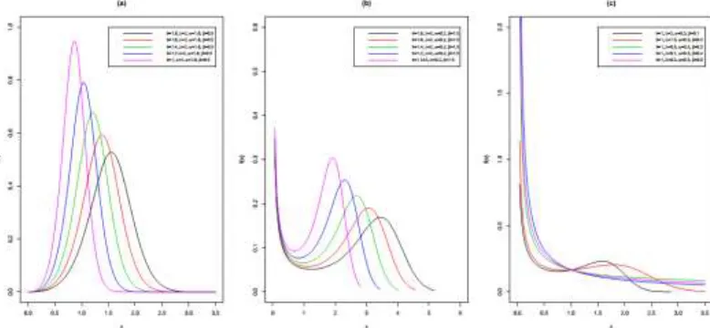
if X is a random variable with density (7), we write X OLLGHNP( , , , )    . Some useful mathematical properties have been transferred to Appendix. Plots of these functions for different values of parameters are shown in Figures 1 , 2 and 3 respectively. It is clear that the new distribution is more flexible than GHN distribution. Fig. 2 displays some plots of the OLLGHNP hrf for some parameter values. It is evident that the hazard rates have four major shapes ascending, descending, unimodal and bathtub. In Figures 3, we plot the measures skewness and kurtosis for the OLLGHNP(1.5,2, ,) distribution, as a functions of  ,. These plots indicate that the skewness always decreases when  increases (for fixed  ) and first decreases steadily to a minimum value and then increases when  increases (for fixed ). The kurtosis always increases when  increases (for fixed ) and increases when  increases (for fixed ). So, the new OLLGHNP distribution is quite flexible and can be used effectively in analyzing real data in many areas.

Figure 2: The OLLGHNP hrf.(a) Unimodal. (b) Increasing. (c) Bathtub form.

Figure 3: Skewness and kurtosis of the OLLGHNP distribution for some values of  and

.

Suppose Z1, ,Zn be independent identically random variables (iid) with common cdf (3) and N be a random variable with,

( )

1

( )

1

( = ) = n exp 1 ! , = 1, 2, , > 1,

P N n  _  − _− n − n 

Define M_N = max(Z₁, ,Z_N) then,

( ) = ( _N )

F x P M x

=1

= ( _N | = ) ( = )

n

P M x N n P N n







( )

1

( )

1 =1

( )

= exp 1 !

( ) ( )

n n n

G x

n

G x G x



   

 _{  − −}

−

 

 ₊   

 

( )

1 ( )

= exp 1 exp 1 .

( ) ( )

G x

G x G x



 



 − −   − 

 _{    }

  _{ + }

 

 

The justification for the practicality of the OLLGHNP lifetime model is based on the fatigue crack growth under variable stress or cyclic load. We also are motivated to introduce the OLLGHNP distribution because it exhibits increasing, decreasing, upside-down as well as bathtub hazard rates as illustrated above; It is shown in Section 3 that the OLLGHNP distribution can be viewed as a mixture of the two-parameter GHN lifetime model; It can be viewed as a suitable model for fitting the the right-skewed, left-skewed and bimodal data as shown in Section 5; The OLLGHNP distribution outperforms several of the well known lifetime distributions with respect to two real data applications as illustrated in Setion 5.

Estimation and Inference

The estimation of the model parameters is performed by the method of maximum likelihood. If X OLLGHNP( , , , )    the vector of parameters is  = ( , , , )    T, the log-likelihood for  from a single observation x of X is given by,

( ) = log(2) log( ) log( ) ( +  +  + −1) log( )x −log( ) log( ) ( + p + −1) log(q−1)

( 1)

( 1) log(2 ) log( 1) 2 log[( 1) (2 ) ],

( 1) (2 )

q q

q e q q

q q



  

 

 −

+ − − + − − − − + −

− + −

where x> 0, p= (( ) ) x 

 and = 2 (( ) )

x

q 



 . The component of the unit score vector

= ( ) = ( , , , )T

U U 

   

   

    are given by,

1

= log(q 1) log(2 q)

 

 _{+ − + −}



2

(2 ) ( 1) log[( 1) (2 ) ]

[( 1) (2 ) ]

q q q q

q q

   

 

 − − − + −

+

− + −

( 1) log( 1) (2 ) log(2 )

2 ,

( 1) (2 )

q q q q

q q

 

 

− − + − −

+

− + −

1 ( 1)

= ,

( 1) (2 ) 1

q e

q q e

    

 

 −

+ −

 − + − −

2

= (( ) 1) ( 1)[ ]

1 2

x

q q



 _  

  

 _{− − − +}

 − −

2 2

( 1) (2 )

[( 1) ( 1) ][( 1) (2 ) ]

q q

q q q q

   

 − −

−

1 1

2 (2 ) ( 1) ]

,

( 1) (2 )

q q

q q

   

 ₋ − _{− −} −

−

− + −

2

= log( / )[1 ( / ) ] ( 1)[ ]

1 2

x x

q q

  

  





− + − +

 − −

1 1 1 1

2

( 1) (2 ) 2 (2 ) ( 1) ]

,

[( 1) (2 ) ] ( 1) (2 )

q q q q

q q q q

   

   

 ₋ − ₋ −  ₋ − _{− −} −

− −

− + − − + −

where

2 2

( ) ( )

2 2

2 2

= ( / ) ( / ) and = log( / ) ( / ) .

x x

e x e x

 

 

 

       

 

− −

For a random sample = ( ,₁ , )T n

x x x of size n from X , the total log-likelihood is

( ) =1

= ( ) = ( )

n i

n n

i





 , where ( )i ( ) is the log-likelihood function for the ith observation

( = 1,..., )i n . The total score function ( )

=1 =

n i n

i

U



U , where U( )i has the form given before

for i= 1,...,n. Maximization of ( ) can be performed using well-established routines such as the nlm or optimize in the R statistical package. Setting these equations to zero,

( ) = 0

U  , and solving them simultaneously gives the MLE, ˆ of  . These equations cannot be solved analytically and statistical software can be used to evaluate them numerically using iterative techniques such as the Newton-Raphson algorithm. For interval estimation and hypothesis tests on the parameters in  , we require the 4 4 unit observed information matrix J = ( ) = {J  j_{r s,}}, whose elements are j_{r s,} for r s, = , , ,    . Under conditions that are fulfiled for parameters in the interior of the parameter space but not on the boundary, the estimated approximate multivariate normal N₄(0,n J−1 ( ) )ˆ −1 distribution can be used to construct approximate confidence intervals for the model parameters. The likelihood ratio (LR) statistics are useful for comparing the new distribution with some special models. For example, we may use the LR statistic to check if the fit using the OLLGHNP distribution is statistically superior to a fit using the GHN distribution for a given data set. In any case, considering the partition  = ( ₁T, ₂T T)

, tests of hypotheses of

the type (0)

0: 1 = 1

H   versus (0)

1 1

: A

H   can be performed using the LR statistic

ˆ

= 2{ ( ) ( )}

w  −  , where ˆ and  are the estimates of  under H_A and H₀,

respectively. Under the null hypothesis H₀, 2 d

q

w→ , where q is the dimension of the parameter vector ₁ of interest. The LR test rejects H₀ if w> , where  denotes the

upper 100 % point of the q2 distribution (Cordeiro et al., 2012).

A simulation study

random sample of size n is drawn from the OLLGHNP( , , , )    distribution and the parameters are estimated by the maximum likelihood method. The random variable X is generated using the inversion method. The true parameter values in the data-generating processes are  = 1.5, = 2,  = 1.8 and  = 1.5.The mean estimates of the four model parameters and the corresponding root mean squared errors (RMSEs) for the sample sizes

n = 50, 100, 150 and 200 are listed in Table 1 and the plot of the corresponding root mean squared errors (RMSEs) for the sample sizes n, equal to 50 to 200 with step 5 are shown in Figure 4. We note that the RMSEs of the MLEs of , ,  and  decay toward zero when the sample size increases, as expected.

Table 1: Mote Carlo simulation results: Mean estimates and RMSEs (in parentheses) of   , , and .

n=50 n=100 n=150 n=200

ˆ

 2.7640(0.6389) 2.2536(0.3040) 1.8551(0.1870) 1.7000(0.0000) ˆ

 1.8360(0.4392) 1.8474(0.2445) 1.9366(0.1388) 2.0000(0.0000) ˆ

 1.3060(0.4124) 1.6052(0.2533) 1.7456(0.1047) 1.8000(0.0000)

ˆ

 1.5245(0.4103) 1.4461(0.2785) 1.4826(0.1254) 1.5000(0.0000)

Real data modeling

In this section, we present application of the OLLGHNP model to real data to illustrate its usefulness and potentiality. We consider two sets of real data and adopt the OLLGHNP distribution as the baseline model. The first real data represents the failure times (in hours) of unscheduled maintenance actions for the USS Halfbeak number 4 main propulsion diesel engine over 25.518 operating hours with 71 observations studied by Ascher and Feingold (1984). It consists of the observations presented in table 2.

Table 2: Diesel Engine Data, Ascher and Feingold (1984)

1.382 9.794 18.122 20.121 21.378 21.815 22.311 23.305 25.000 2.990 10.848 19.067 20.132 21.391 21.820 22.634 23.491 25.010 4.124 11.99319.172 20.431 21.456 21.822 22.635 23.526 25.048 6.827 12.300 19.29920.525 21.461 21.888 22.669 23.774 25.268 7.472 15.413 19.360 21.05721.603 21.930 22.691 23.791 25.400 7.567 16.497 19.686 21.061 21.65821.943 22.846 23.822 25.500 8.845 17.352 19.940 21.309 21.688 21.94622.947 24.006 25.518 9.450 17.632 19.944 21.310 21.750 22.181 23.14924.286

The source of the second data set is the open university. The following data are the prices of the 31 different children’s wooden toys on sale in a Suffolk craft shop in April 1991: 4.2, 1.12, 1.39, 2, 3.99, 2.15, 1.74, 5.81, 1.7, 2.85, 0.5, 0.99, 11.5, 5.12, 0.9, 1.99, 6.24, 2.6, 3, 12.2, 7.36, 4.75, 11.59, 8.69, 9.8, 1.85, 1.99, 1.35, 10, 0.65, 1.45. We compare the proposed model with the following lifetime distributions: Odd Log-Logistic Generalized Half-Normal(OLLGHN) distribution (Gauss M. Corderio. et al., 2016), Beta Generalized Half-Normal Geometric (BGHNG) distribution (Thiago G. et al., 2013), Beta Generalized Half-Normal (BGHN) distribution (Pescim et al., 2010), Exponentiated Generalized Half-Normal (EGHN) distribution (Pescim et al., 2010), Kumaraswamy Generalized Half-Normal (KwGHN) distribution (Cordeiro et al., 2012), Marshall-Olkin Generalized Half-Normal (MOGHN) distribution (Alizadeh et al., 2015) and Generalized Half-Normal (GHN) distribution (Cooray and Ananda, 2008).

For each model, we estimate the unknown parameters by using maximum likelihood approach. The computations were done using the statistical software R. Table 3, gives the maximum likelihood estimation (MLE) of the model parameters and their standard errors (in parentheses) and the values of the following statistics for the fitted models by using the first set of real data and Table 6 for the second: Akaike Information Criterion (AIC= 2p−2log( )L ), Bayesian Information Criterion (

= log( ) 2log( )

distributions considered in Table 4 (for the first data) and Table 7 (for the second data) and therefore it can be an interesting alternative to these distributions for modeling each of the real data set. Comparisons of the OLLGHNP distribution with GHN, GHNP(submodel of OLLGHNP when  =1) and OLLGHN distributions individually (that has less than four parameters) using the LR statistics are given in table 5 (for the first data) and table 8 (for the second real data). We reject the null hypotheses of the LR tests in favor of the OLLGHNP distribution.

Table 3: MLEs and standard errors (in parentheses) and the AIC and BIC statistics for the first real data

Model Estimates Statistics

AIC BIC

OLLGHNP 16.6264 4.3495 0.2284 3.1954 397.7 406.7 -1.1556 -0.6238 -0.065 -0.7559

OLLGHN 20.5159 7.2435 0.3189 414.1 420.9 -0.5716 -0.9632 -0.065

BGHNG 18.3336 6.1205 0.2963 0.0953 0.2033 405.1 416.5 -0.024 -0.0238 -0.0592 -0.0234 -0.3129

BGHN 19.9467 8.4713 0.2121 0.1137 404.1 413.2 -0.004 -0.004 -0.0353 -0.0154

EGHN 24.4685 11.94 0.244 419.7 426.5 -0.0049 -0.0049 -0.029

KwGHN 19.0036 6.9884 0.1164 0.1172 399.4 408.4 -0.0042 -0.0058 -0.0116 -0.014

MOGHN 15.8886 2.2263 14.8719 419.2 425.9 -1.7863 -0.4248 -9.9684

GHN 21.8836 3.8205 438.5 443 -0.497 -0.415

Table 4: Formal goodness of fit tests for the first real data.

Model Statistics

*

W A*

OLLGHNP 0.0714 0.4543

OLLGHN 0.3282 1.6439

BGHNG 0.1269 0.7228

BGHN 0.2050 1.0790

EGHN 0.4870 2.4889

KwGHN 0.0982 0.5956

MOGHN 0.3830 2.1090

Hypothesis Statistics w p-value

0: 1:

H GHN vs H OLLGHNP 44.80 0.0000

0: 1:

H GHNP vs H OLLGHNP 33.72 0.0000

0: 1:

H OLLGHN vs H OLLGHNP 18.47 0.0000

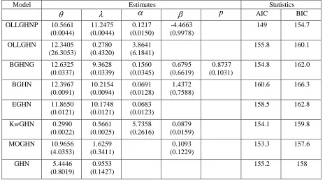
Table 6: MLEs and standard errors (in parentheses) and the AIC and BIC statistics for the second real data.

Model Estimates Statistics

    p AIC BIC

OLLGHNP 10.5661 (0.0044)

11.2475 (0.0044)

0.1217 (0.0150)

-4.4663 (0.9978)

149 154.7 OLLGHN 12.3405

(26.3053)

0.2780 (0.4320)

3.8641 (6.1841)

155.8 160.1 BGHNG 12.6325

(0.0337)

9.3628 (0.0339)

0.1560 (0.0345)

0.6795 (0.6619)

0.8737 (0.1031)

154.8 162.0 BGHN 12.3967

(0.0091)

10.2154 (0.0094)

0.0691 (0.0128)

1.4372 (0.7588)

160.6 166.3 EGHN 11.8650

(0.0121)

10.1748 (0.0121)

0.0683 (0.0123)

158.5 162.8 KwGHN 0.2990

(0.0022)

0.5661 (0.0025)

5.7358 (0.2616)

0.0879 (0.0159)

154.1 159.8 MOGHN 10.9656

(4.0353)

1.6259 (0.3411)

0.1093 (0.1229)

153.3 157.6 GHN 5.4446

(0.8019)

0.9553 (0.1427)

155.2 158

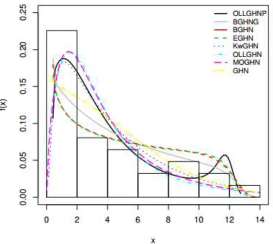
Figure 5: The histogram of first real data with the fitted density functions.

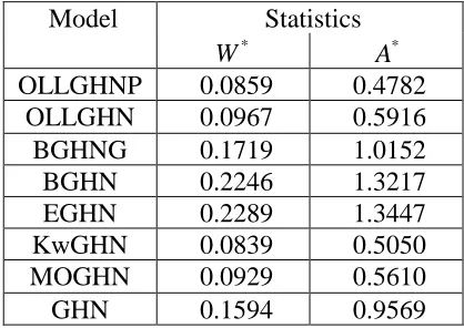
Model Statistics

*

W A*

OLLGHNP 0.0859 0.4782

OLLGHN 0.0967 0.5916

BGHNG 0.1719 1.0152

BGHN 0.2246 1.3217

EGHN 0.2289 1.3447

KwGHN 0.0839 0.5050

MOGHN 0.0929 0.5610

GHN 0.1594 0.9569

Table 8: LR tests for second real data.

Hypothesis Statistics w p-value

0: 1:

H GHN vs H OLLGHNP 10.22 0.0060

0: 1:

H GHNP vs H OLLGHNP 8.93 0.0028

0: 1:

H OLLGHN vs H OLLGHNP 8.82 0.0030

Conclusions

The odd log-logistic generalized half-normal (OLLGHN) distribution is commonly used to model the lifetime of a system. We propose a new four parameter model called the odd log-logistic Poisson generalized half-normal (OLLGHNP) distribution, whose failure rate function can be increasing, decreasing and bathtub that extends the OLLGHN (Gauss M. Corderio. et al., 2016), MOGHN (Alizadeh et al., 2015), EGHN (Pescim et al., 2010), generalized half-normal (GHN) and half-normal (HN) (Cooray and Ananda, 2008) distributions. The OLLGHNP distribution is quite flexible in analyzing positive data in place of some other special models. We provide an expansion for the density function and a mathematical treatment of the distribution including expansions moments and generating function. The estimation of the model parameters is approached by the method of maximum likelihood and a simulation study is performed. We consider likelihood ratio statistics and formal goodness-of-fit tests to compare the OLLGHNP distribution with some other lifetime models that include four, less than four and more than four parameters. Applications of the new model to two real data sets individually demonstrated that it can be used effectively to provide a more suitable fit than other models. We hope that this generalization can find wider applications in the literature of lifetime distributions.

Acknowledgment

The authors would like to thank the referees and editor for supplying extremely helpful comments and suggestions.

References

2. Aarts, R.M. (2000). Lauricella functions, www.mathworld.com/LauricellaFunctions.html. From MathWorld - A Wolfram Web Resource, created by Eric W. Weisstein.

3. Alexander, C., Cordeiro, G.M., Ortega, E.M.M. and Sarabia, J.M. (2012). Generalized beta- generated distributions, Computational Statistics and Data Analysis, 56, 1880-1897.

4. Alizadeh, M., Cordeiro, G.M., Brito, D.E., and Demtrio, C.G.B. (2015). The beta Marshall-Olkin family of distributions, Journal of Statistical Distributions and Applications, 2:4, DOI 10.1186/s40488-015-0027-7. particle counts, "Semiconductor International, June, 117-122.

5. Ascher, H. and Feingold, H. (1984). Repairable Systems Reliability, Marcel Dekker, New York.

6. Chen, G. and Balakrishnan, N. (1995). A general purpose approximate goodness-of-fit test, Journal of Quality Technology, 27, 154-161.

7. Cooray, K. (2006). Generalization of the Weibull distribution: the odd Weibull family, Statistical Modeling, 6, 265-277.

8. Cooray, K. and Ananda, M.M.A. (2008). A Generalization of the HalfNormal

Distribution with Applications to Lifetime Data, Communication in Statistics - Theory and Methods, 37, 1323- 1337.

9. Cordeiro, G.M., Alizadeh, M., Pescim, R.R. and Ortega, E.M.M. (2016). The odd log-logistic generalized half-normal lifetime distribution: properties and applications, Communications in Statistical-Theory and Methods, 4195-4214.

10. Cordeiro, G.M., Alizadeh, M., Pescim, R.R. and Ortega, E.M.M. (2016). The odd log-logistic generalized half-normal lifetime distribution: properties and applications, Communications in Statistical-Theory and Methods, 4195-4214.

11. Cordeiro, G.M. and Lemonte, A.J. (2011). The beta Birnbaum Saunders distribution: An im- proved distribution for fatigue life modeling, Computational Statistics and Data Analysis, 55, 1445-1461.

12. Cordeiro, G.M., Lemonte, A.J. and Ortega, E.M.M. (2013). An extended fatigue life distribution, Statistics, 47, 626-653.

13. Cordeiro, G.M., Ortega, E.M.M., Lemonte, A.J. (2014). The exponential Weibull lifetime distribution, Journal of Statistical Computation and Simulation, 47, 626-653.

14. Cordeiro, G.M., Pescim, R.R. and Ortega, E.M.M. (2012). The Kumaraswamy Generalized Half- Normal Distribution for Skewed Positive Data, Journal of Data Science, 10, 195-224.

16. Merovci, F., Alizadeh, M., Yousof, H. M. and Hamedani G. G. (2017). The exponentiated transmuted-G family of distributions: theory and applications, Communications in Statistics-Theory and Method, forthcoming.

17. The Open University. MDST242 Statistics in Society Unit A0: Introduction . 2nd ed.,Milton Keynes: The Open University,1963, Table 3.1.

18. Trott, M. (2006). The Mathematica Guidebook for Symbolic. With 1 DVD-ROOM (Windows, Macintosh and UNIX). Springer, New York.

Appendix A

First, we define the exponentiated-G (“ Exp-G” ) distribution for an arbitrary parent distribution G x( ), say W Expc( )G , if W has cdf and pdf given by ( ) = ( )c

c

H x G x and

1

( ) = ( ) ( )c ,

c

h x cg x G x − respectively. This transformed model is also called the Lehman type I distribution, say Expc( )G . For c> 1 and c< 1 and for larger values of x, the multiplicative factor cG x( )c−1 is greater and smaller than one, respectively. The reverse assertion is also true for smaller values of x. The latter immediately implies that the ordinary moments associated with the density function h xc( ) are strictly larger (smaller) than those associated with the density g x( ) when c> 1 (c< 1). Second, with using Taylor expansion for the cdf of OLLGHNP we obtain,

( )

1

( )

1

=0

( ) = exp 1 ! 2 1

i i

i

x

F x i

 

 

 

− −     

−  −

      

  _{ }

 

   

 



2 1 2 2 .

i

x x

 

 

 

− _{        } 

 

 _ _{  }− _ +_ − _{  } _{        } 

 

(A1)

Now, we obtain an expansion for F x( ). First, we use a power series for G x( ) ( > 0 real) given by,

=0

( ) = ( ) 2 1 ,

k

k k

x

G x a



 _



 _ _{ }  _

_{ }−   _{ } 

 

   

 



(A2)

where,

=

( ) = ( 1)k j .

k

j k

j a

j k    ₋ +   

     



For any real > 0, we consider the generalized binomial expansion

=0

2 2 = ( 1) 2 1 .

k k

k

x x

k 

 _ 

 



   _{ }   

 _{− }    ₋  _   ₋ 

   

  _{ }     _{ } 

 

   

      

 



  (A3)

=0

=0

2 1 ( ) 2 1

= ,

2 1

2 1 2 2

i k k k i k k k x x a i x

x x _b

                         _   ₋   _   ₋        _{ }    _{ }                  _{        }  _ _{ }  _  −    −  + −       _{ }                  





where b_k =h_k( , ) i is defined in Appendix B. The ratio of the two power series can be expressed as,

=0

=0

=0

( ) 2 1

= 2 1 ,

2 1 k k k k k k k k k x a i x c x b                _   ₋        _{   }               _{  − }              _   ₋                 







(A4)

where the coefficients c_k’s (for k0) are determined from the recurrence equation,

1 1

0 0

=1

= ,

k

k k r k r

r

c b− _a −b− b c ₋ _







then we can write,

=0

( ) = _{k k}( ),

k

F x d H x





(A5)

where,

( )

1

( )

1

=0

= exp 1 i ! ( , )for 0.

k k

i

d   i c  i k



− −

− 

 

 



The pdf of X follows by differentiating (A5) as,

1 1

=0

( ) = k k ( ),

k

f x d h x



+ +



(A6)

where ₁( ) = ( 1) ( )k ( ) k

h₊ x k+ G x g x is the Exp-G density function with power parameter

(k+1). Equation (A6) reveals that the OLLGHNP density function is a linear combination of Exp-GHN densities. Thus, some structural properties of the new family such as the ordinary and incomplete moments and generating function can be immediately obtained

from well-established properties of the Exp-GHN distribution.By setting u= x



       and

considering the error function as the cdf of the GHN distribution, the nth moment of X

can be obtained from equation (A6) as,

( )

(

)

1 2 1 =0 2 = = / , ,

' n n

n k

k

E X b I n k

     +      



where,

(

)

2

0

1

/ , = exp ,

2 2

k n

u

I n  k u u erf du

 _{  }

₋ 

        

( )

( )

(

2

)

1

=0 1 2

= ,

! 2 1

m m m x erf x m m  +  ₋ +



in the last equation and computing the integral, we have (for any real k+n/) we get,

( )

(

)

1 2 1 =0 2 = / , , n n k k

E X  b I n  k   +      



inserting the power series for the error function,

( )

( )

(

2

)

1

=0 1 2

= ,

! 2 1

m _m m x erf x m m  +  ₋ +



in the last equation and computing the integral, we have (for any real k n



+ ) we get,

( )

(

)

1 2 1 =0 2 = / , , n n k k

E X  b I n  k   +      



where,

(

)

12 2 12

( )

1 ...

,..., =0 1 2 1

1

/ , = 2

! !... !

m m

n k

k k

m m_k k

I n k

m m m

   + +  − + + − −



(

)

1

1 2

1

1 / ...

2

.

1 1 1

...

2 2 2

k

k

k n m m

m m m

   _ _ + + _+ + + _     ₊  ₊   ₊           

Moreover, for the very special case when k+n/ is even, the integral I n

(

/ , k

)

can be expressed in terms of the Lauricella function of type A (Exton, 1978; Aarts, 2000) defined by

( )

(

)

1

1

1 1 1

=0 =0 1

1 ... ; ,..., ; ,..., ; ,..., = ... !... ! m m _n n n

A n n n

m m_n n

x x F a b b c c x x

m m  

 

( )

( )

( )

( )

( )

( )

1 1 1 ... ... , ...

m m_n m m_n

m m_n

a a b b

c c

+ + + + +



+ +

where

( )

= k

a a a

(

+1 ...

) (

a k+ −1

)

is the ascending factorial (with the convention that

( )

a ₀ = 1). Numerical routines for the direct computation of the Lauricella function of type A are available, see Exton (1978) and Mathematica (Trott, 2006). Hence,

( )

n

E X can be

expressed in terms of the Lauricella functions of type A,

( )

( )

1 2

=0

2 1 1 1 3 3

= 1 ; ,..., ; ,..., ; 1,..., 1 ,

2 2 2 2 2

k

n n

k A k

n

E X   F k

   _{ }    _{+ +}  _{− −}        



    where, 1 1

2 2 2

1

1

= 2 1 .

The central moments (_n) and cumulants (_n) of X are determined using E X

( )

n as,

1 =0

= ( 1)

n

k 'k '

n n k

k

n

k

  _{ } −   ₋

 



and,

1 =1 1 = , 1 n ' '

n n k n k

k n k   − − _ − _  ₋ −  



respectively, where ₁=₁'. The skewness ₁ = ₃/ ₂3/2 and kurtosis ₂ = ₄ / ₂2 are obtained from the third and fourth standardized cumulants. The moment generating function (mgf) of of X, say MX

( )

t =E e

( )

tX ,is given by,

( )

( )

=0

= n n / !.

X n

M t t E X n





The characteristic function (cf) of X , 

( )

t = E e

( )

it X , and the cumulant generating function (cgf) of X , K t

( )

= log

( )

t can be obtained from the well known relationships, where i= −1.

Appendix B

We present three power series expansions required for the proof of the general result in Appendix A. By expanding z in Taylor series, we can write

=0 =0 ( 1) = ( ) = , ! k i k i k i z

z f z

k 



 − _



 (B1) where = ( 1) = ( ) = ( ) ! k i

i i _{k i} k

k f f i k   − −       



and ( ) = ( _k  −1) (− +k 1) is the

descending factorial. Further, we obtain an expansion for [ ( )a ( ) ]a c

G x +G x . We can write,

=0

( )a ( ) ] =a _j ( ) ,j j

G x G x t G x 

+



where,

= ( ) = ( ) ( 1)j .

j j j

a t t a a a

j

  + − _{ }  

Then, using (A1), we have,

=0 =0

( ) ( ) ] = ( ) ,

i

a a c j

i j

i j

G x G x f t G x

 _  _

+ _{ }

 

 

where f_i = f c_i( ). Finally, we obtain,

=0

( )a ( ) ] =a c _j( , ) ( ) ,j j

G x G x h a c G x  +



where, , =0 ( , ) =

j i i j

i

h a c f m





and for i0 _, = ( ₀) 1 [ ( 1) ] _, (for 1)and _,0 = .₀ j

i

i j m i j m i