* Corresponding author
E-mail: [email protected] (R. Matindi) 2019 Growing Science Ltd.
doi: 10.5267/j.ijiec.2018.5.003
International Journal of Industrial Engineering Computations 10 (2019) 17–36
Contents lists available at GrowingScience
International Journal of Industrial Engineering Computations
homepage: www.GrowingScience.com/ijiec
Developing a versatile simulation, scheduling and economic model framework for bioenergy production systems
Robert Matindia*, Phil Hobsona, Mahmoud Masoudb, Geoff Kenta and Shi Qiang Liuc
aSchool of Chemistry, Physics and Mechanical Engineering Science and Engineering Faculty, Queensland University of Technology, Brisbane Qld 4001 Australia
bSchool of Mathematical Sciences, Queensland University of Technology, 2 George St, Brisbane Qld 4001 Australia cSchool of Economics and Management, Fuzhou University, Fuzhou, 350108, China
C H R O N I C L E A B S T R A C T
Article history:
Received January 30 2018 Received in Revised Format February 18 2018
Accepted May 28 2018 Available online May 28 2018
Modelling is an effective way of designing, understanding, and analysing bio-refinery supply chain systems. The supply chain is a complex process consisting of many systems interacting with each other. It requires the modelling of the processes in the presence of multiple autonomous entities (i.e. biomass producers, bio-processors and transporters), multiple performance measures and multiple objectives, both local and global, which together constitute very complex interaction effects. In this paper, simulation models for recovering biomass from the field of the biorefinery are developed and validated using some industry data and the minimum biomass recovery cost is established based on different strategies employed for recovering biomass. Energy densification techniques are evaluated for their net present worth and the technologies that offer greater returns for the industry are recommended. In addition, a new scheduling algorithm is also developed to enhance the process flow of the management of resources and the flow of biomass. The primary objective is to investigate different strategies to reach the lowest cost delivery of sugarcane harvest residue to a sugar factory through optimally located bio-refineries. A simulation /optimisation solution approach is also developed to tackle the stochastic variables in the bioenergy production system based on different statistical distributions such as Weibull and Pearson distributions. In this approach, a genetic algorithm is integrated with simulation to improve the initial solution and search the near-optimal solution. A case study is conducted to illustrate the results and to validate the applicability for the real world implementation using ExtendSIM Simulation software using some real data from Australian Mills.
© 2019by the authors; licensee Growing Science, Canada
Keywords:
Bio-refinery Cane harvesting Supply chain Genetic algorithm
1. Introduction
(coal, petroleum and natural gas), resulting in over 8.5 Gt C/year of carbon dioxide emissions (Gregg & Smith, 2010 p241).
Global consumption of fossil fuels is expected to increase by 57% from 390EJ to 610 EJ, which will cause a 58% rise in energy-related emissions from 26.6 to 41.9 Gt CO2E between 2005 and 2030 (Resch
et al., 2008 p4048). Furthermore, economic and population growth continue to be the most important global drivers of increase in CO2 emissions from fossil fuel combustion. The growth in population has
largely remained the same between 2000 and 2010, while the economic growth continued to rise. Continued use of coal based fuels has effectively reversed the gains of gradual decarbonisation (i.e., reducing the carbon intensity of energy) of the world’s energy supply. Based on equity principles, industrialized countries must reduce their emissions by a greater amount - 80% below 1990 levels by 2050 (Rivers & Jaccard, 2005 p307).
Due to the mentioned challenges, there is an urgent need for research into technologies for conversion of lignocellulosic biomass into liquid transportation fuels and other products and a number of studies have been perfomred recently focussing on various aspects that need to be optimised in bioenergy production, (Farine et al., 2012 p148; Sims et al., 2010 p1570; Dias et al., 2012 p152; Meyer et al., 2012 p1). Among the findings from the above studies, the inflexion point to profitability and net present worth of such projects rely on supply curve costs. The costs have previously been studied and demonstrated to be a function of spatial concentration, and bulk density, unlike their equivalent in the supplementary industry (Petroleum industry) where oil wells are the source of feedstock (Brinsmead et al., 2015 p21).
For many conversion technologies, biomass needs to be harvested/recovered and transported to a centralised or decentralised bio refinery or energy plant for conversion into higher value products (fuels, energy). The combined result of the dispersed nature of biomass feedstock and the integration of various conversion technologies, for the purposes of energy densification, is that the total feedstock price becomes heavily dominated by the transportation and the value place of feedstock on the ground.
The recovery of feedstock therefore must balance the competing interests in the bioenergy sector; which are for the feedstock producers (mostly the agronomic interests), the bio processors (the transportation and conversion process), and the whole industry (the project viability) and the trade-off between the competing uses must guarantee returns not only to the feedstock producers, but also the bio processors.
In order to comprehensively address the shortcomings in the bioenergy production systems, system optimisations ranging from new scheduling algorithms for trucks and locomotives are developed in this study to improve the makespan for a conceptual biorefinery transport system. Further, using simulation optimisation technique; the minimum cost of biomass recovery in context of sugarcane industry is established, energy densification and conversion technologies are further been evaluated so that the net present worth cane of different pre-treatment and processing technology can be established.
2. Research Problem
R. Matindi et al.
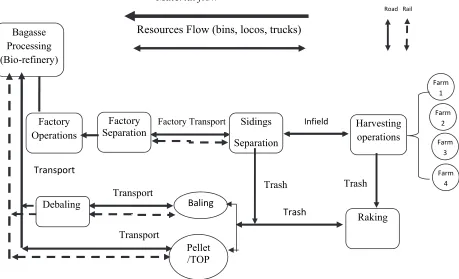
and leaf fibre, and resources such as harvesters, locomotives and bins. These five main stages include harvesting, infield transport, factory transport, factory operations and bagasse processing.
Material flow
Resources Flow (bins, locos, trucks) Fig. 1. Existing sugarcane biomass supply chain
Fig. 2 shows the modified sugarcane supply chain including new selected stages where trash could potentially be recovered and depicts the overall impact and the recovery process on the industry. The new process stages added to the previously existing sugarcane supply chain where new stages are: Partial harvester separation, factory separation, post-harvest raking and baling process, Pelletisation (Energy densification), Torrefaction (Energy densification), debaling and storage of bagasse, pellets/Briquettes, Torrefied Pellets, (TOP), and trash and their implication in the existing industry set up.
Material flow
Resources Flow (bins, locos, trucks)
Fig. 2. Modified sugarcane biomass supply chain
Harvesting
Operations Farm3
Farm 2 Farm
1
Farm 4
Infield Transport Factory Transport
Bagasse Processing (Bio-refinery)
Factory Operations
Harvesting
operations Farm
3 Farm
2 Farm
1
Farm 4 Infield
Factory Transport
Bagasse Processing (Bio-refinery)
Factory Operations
Trash
Trash Baling
Pellet /TOP
Trash
Raking Sidings
Separation
Debaling Transport
Transport
Factory Separation
Transport
Road Rail
The technical operating parameters for factory trash separation are based on a post-harvest cane cleaning technology in terms of leaf removed/leaf remaining, cane loss and power consumption systems. The extension of the economic overlay will be based on the apportion cost on the new processes that have been added or modified in the supply chain (supply chain segments impacted by trash recovery) which includes: siding separation, factory separation, raking and baling process, pelletising transportation of pellets and bales, debaling and storage of bagasse or pellets and trash.
Supply chain costs remain the major impediment for large-scale biomass when competing with fossil fuels (Gan & Smith, 2006 p296). In wood-based energy production, for instance, it is difficult to achieve the same economies of scale as the fossil fuels because of the disadvantages of transporting widely distributed biomass to a central location. This will in effect negatively impact the economic sustainability of wood-based energy production (Ranta et al., 2012 p33). The price of the biomass is highly variable due to its low energy content and transport economies and thus the need for improvement in the productivity of biomass production, harvesting, and transport systems and conversion technology (end to end supply chain) is the key for enhancing the bioenergy share of total energy production (Gan & Smith, 2006 p296).
When availability and supply chain costs are aggregated, the cumulative availability, total costs and marginal cost of biomass supply can be calculated (Asikainen et al., 2008). The costs and availability of woody biomass vary largely in different countries. From an economical perspective, optimal stands for biomass harvesting should have a high density (m3 ha-1) of harvestable biomass, forwarding distance
should be less than 500 meters and long distance transportation should be less than 100 kilometres (Raulund-Rasmussen et al., 2008 p29). This however, is seldom the case in reality particularly in the sugar industry where the sidings have been set to distances beyond the recommended forwarding distance. Remote areas may not be economically suitable for harvesting due to higher transportation costs but if demand increases these resources may have to be utilized. As biomass is transported further, more transportation fuel is used (Ikonen et al., 2013 p1).
Different scenarios are addressed in this paper to optimise the harvesting operations using innovative approaches. The economic overlay will cover three potential scenarios of feedstock recovery process. The model postulates that some of the simulated outputs from the system at various stages are; the “biomass type” with various attributes, where the type in this context refers to biomass from sugarcane industry which essentially are the cane residue, and bagasse. These biomass types can be densified further briquettes or torrefied biomass depending on the economics involved. The economic model (financial overlay) developed consequently put a cost against a scenario where trash is transported to the mill/biorefinery as part of normal cane supply using the current mill transport system (Whole of cane harvesting with factory feedstock recovery), other recovery procedure entails raking and baling, torrefaction and Pelletisation. The proposed scenarios are:
Scenario 1: After cane harvesting, the trash left infield is baled and transported to the mill and mixed with surplus bagasse stream for storage and bioenergy production.
Scenario 2: The cane harvester is operated with the with fans turned off in the harvester cleaning chamber, the trash is transported to the mill together with the cane and the trash/cane separation process takes place in the cane cleaner installed at the mill.
Scenario 3: The cane harvester is operated with the fans turned off in the harvester cleaning chamber, the trash is transported to the mill together with the cane and the trash/cane separation process takes place in the cane cleaner installed at the mill, the separated trash is further densified to briquettes.
R. Matindi et al.
2.1 Feedstock type and recovery operations under investigation
2.1.1Sugarcanefibre(fromcaneresidue)
The total cost for recovery of agricultural residues are regio-specific and thus their costs are highly variable. Some practical approaches for their recovery as opined by Hobson et al. (2006 p1) and Thorburn et al. (2006 p27) in their studies largely fall into two categories as follows,
i. Rake and bale process as a post harvest operation
ii. Full cane harvesting with factory separation of trash from billet at the mill.
Historically, the drivers of sugar industry have been the clean cane, and sugar recovery process with little emphasis on the value of trash, thus the actual cost for large commercial operation of trash recovery are not well understood, studied or known. Previous studies (Thorburn et al., 2005 p1) did a comparison between the whole of cane harvesting and raking and baling using and they found out that the cost was more than half the cost of raking and baling. Thus, in order to determine the cost of biomass being recovered, the cost of the whole of cane harvesting, forms the lower limit of the cost of cane residue, the cost of raking and baling forms the median cost, while pelletisation, Torrefaction or Torrefaction and pelletisation forms the upper limit for the cost of cane residue, this forms a further extension of the study by Hobson and Ridge (2000 p1). The whole of cane supply costs are adopted from Thorburn et al. (2007) and corrected using CPI. The changes in cost and revenues are staggered into the following components:
The Agronomic costs The harvesting costs Rail/Road transport costs, Amortised cane feeding costs Amortised crushing costs Factory separation costs
Net returns /Nil returns from power sales Total return from sugar and molasses And the value of cane supplied.
The approach used by Thorburn et al. (2006 p27) in evaluating the net benefits of whole of crop harvesting has been adopted in this study, and this entailed simulating cost extrema based on the value placed on the trash in those regions. Some regions burn trash in order to facilitate the irrigation processes, that would otherwise impede the irrigation process, while others, retain trash blanket in order to reduce soil erosion and reduce minimise the loss of moisture. Some of the impact being investigated is the trade off between the agronomic costs occasioned by loss of yield as a result of removing trash against the bioprocessors acquiring that trash for biomergy production.
From this study, it was established that recovery cost of feedstock from the two cost extrema were a range of 9.73 $/GJ and 14.18 $/GJ lower and upper limit, respectively.These limits in effect represented regions that burn off trash and the those which would not be in that order.
2.1.2 Rake and Baling Process
In simulating the baling process, the ExtendSIM model generates items (the cane daily allotment (tonnages) that a harvester needs to harvest during the season, the trash in this scenario is cleaned at the harvester and left on the ground. After the cane harvester finishes harvesting a given block of cane, the baler with raking and windrowing capabilities is sent to the block to rake and bale the trash left behind by the harvester. The baled cane is dropped in a row where a bale collector/stacker, collects all the bales and delivers them to the siding, at the siding, the bales are unloaded and stack at the siding, or any other pre-treatment area, where a waiting flatbed trailer is loaded and transport then bales to the biorefinery.
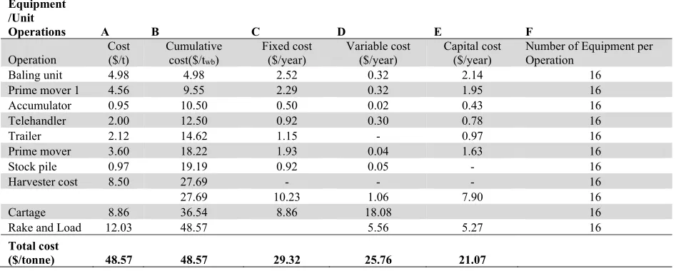
At the biorefinery, the bales are unloaded and stored and only a portion needed for the factory start up and daily production of bio-power or bioenergy. Table 1 shows the various cost factors and operations that goes to the recovery of feedstock using raking and baling process which covers the equipment and the processes involved i.e. prime mover and baler operation, Bale stacker and zone loading operations, prime mover and main transport operations.
Table 1
Summary of the cost of recovering, baling, and stacking cane residue bales Equipment
/Unit
Operations A B C D E F
Operation
Cost ($/t)
Cumulative cost($/twb)
Fixed cost ($/year)
Variable cost ($/year)
Capital cost ($/year)
Number of Equipment per Operation
Baling unit 4.98 4.98 2.52 0.32 2.14 16
Prime mover 1 4.56 9.55 2.29 0.32 1.95 16
Accumulator 0.95 10.50 0.50 0.02 0.43 16
Telehandler 2.00 12.50 0.92 0.30 0.78 16
Trailer 2.12 14.62 1.15 - 0.97 16
Prime mover 3.60 18.22 1.93 0.04 1.63 16
Stock pile 0.97 19.19 0.92 0.05 - 16
Harvester cost 8.50 27.69 - - - 16
27.69 10.23 1.06 7.90 16
Cartage 8.86 36.54 8.86 18.08 16
Rake and Load 12.03 48.57 5.56 5.27 16
Total cost
($/tonne) 48.57 48.57 29.32 25.76 21.07
To be noted, the variable costs of a machinery are calculated from the variable rate by the actual number of hours that a machine runs in order to complete a given unit operation, whereas the fixed rate, a fixed number of operating hours are always postulated for the machine, and this is normally annual rate (a fixed number of useful hours). The capital cost is the ownership requirements for a given equipment, or the custom hire rate.
The simulated region had 128501 tonnes of trash that were recovered over a period of 125 days, the minimum number of equipment required to recover, all the trash through rake and bale within the stipulated timelines are also outlined.
The net returns from the above scenarios are quantified using incremental analysis starting from the baseline, the minimum cost of feedstock is obtained for each technology alternative, which equates to the minimum cost of feedstock at the factory gate. This in effect implies, the factory reconfigures it existing array of equipment predominantly installed to recover sugar, and expand it to accommodate bioenergy production, the required equipment are costed, and amortised over the biomass recovered.
2.2 Transport Operations
R. Matindi et al.
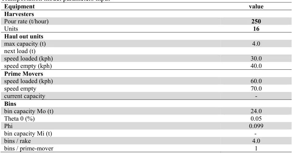
computed together with that of the harvester as a unit. The second form of transportation within the sugarcane industry is from the sidings to the mill/biorefinery. The simulation set up for the current industry, in terms of prime movers, bins and locos used as stipulated in Table 2 and Table 3 below gives the resources performance metrics and the type of resources needed in order to simulate the biomass recovery and transportation to the biorefinery. The components are inputs to the technical model, which then output the required numbers of resources based on the assumption of the input parameters and the quantity of biomass recovered for a given region.
Table 2
Transportation model parameters input
Equipment value
Harvesters
Pour rate (t/hour) 250
Units 16
Haul out units
max capacity (t) 4.0
next load (t)
speed loaded (kph) 30.0
speed empty (kph) 40.0
Prime Movers
speed loaded (kph) 60.0
speed empty 70.0
current capacity -
Bins
bin capacity Mo (t) 24.0
Theta 0 (%) 0.05
Phi 0.099
bin capacity Mi (t) -
bins / rake 4.0
bins / prime-mover 1
Table 3
Resources Management inputs
Description value
Haul out units 12.0
Bins 1000.0
Locomotives 4.0
Prime-movers 30.0
Harvesters 30
The blank space shown with “-” on the table are the output from ExtendSIM model that gets filled in after every simulation run, the effect of trash (cane residue) on the transportation economics was simulated by checking the effect of changing payload as the amount of cane residue in the supply increased or decreased. In order to model the decrease in bin weight as trash in cane increases, the following relationship is used (Tully Model)
3.84 0.09 % , (1)
The bulk densities consequently affect the transport requirements and costs, because they determine the maximum payloads transported, which in terms of simulation output leads to a higher increase in the resources being used (i.e. increase in number of bins, trucks, and prime movers). When transporting sugarcane the model adjusts the expected payload by a factor depending on whether it is green sugarcane or burnt sugarcane.
The proposed mathematical models include Model 1 which describes the maximisation of net gain in sugarcane production; Model 2 which examines the viability of producing cane and trash simultaneously; and Model 3 which seeks to maximises net return by investigating the profitability of harvesting cane green and leaving the trash for raking and baling as a separate operation.
3. Solution Approach
This research presents a novel scheduling model of scheduling N jobs (trips) on M parallel machines (harvesters) that minimizes bi-objectives, namely the total operating time of trips of train/trucks and the total waiting times of all harvesters and mill for empty and full bins. The trips have some precedence relations with different release and due dates. As the sequence-dependent setup times must be determined in the model, it is intractable to solve the large-scale instances to exactitude.
A simulation/optimisation model of the sugarcane harvesting and delivery systems based on a particular mill and its supply area was developed. The purpose of the model was to study methods of reducing harvest-to-crush delays in the sugar industry whilst also reducing the associate costs for biomass supply chain. The use of simulation modelling made it possible to model such a complex system in which all the components of the harvesting and delivery system were integrated so that a holistic view of the system could be obtained to address the interests of both biomass producers and the millers. Furthermore, the proposed system seamlessly links the recovery, transport, processing and storage of feedstock in the biorefinery. The model considers the time-dependent events which are associated with the operating capacities of equipment and storage units. Biomass quality was measured on the amount of moisture, and ash content, which has an effect on the production process, as they both acts as fuel diluents. In the content of developing a scheduling system, biomass supply and demand in this scenario are treated as stochastic variables.
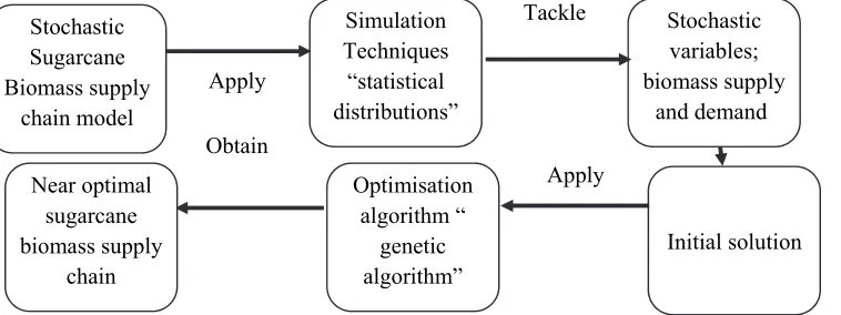
3.1 Hybrid Simulated annealing /Genetic Algorithm
Given the importance of devising faster methods to obtain near-optimal solutions to the transport cane scheduling problems, a lot of works have been accomplisged into developing such techniques using tools like Tabu Search and Simulated Annealing (Masoud et al., 2015 p2569; Masoud et al., 2016 p211). In this research, a hybrid Simulated Annealing/Genetic Algorithm is developed to optimise stochastic biomass supply chain using multi objective functions (minimizing total waiting times for bin and minimizing total operating time for all transport systems (road/rail)).
Fig. 3. Hybrid Simulated Annealing/Genetic Algorithm for biomass supply chain
Stochastic Sugarcane Biomass supply
chain model
Simulation Techniques “statistical distributions”
Stochastic variables; biomass supply
and demand
Initial solution Optimisation
algorithm “ genetic algorithm” Apply
Tackle
Produce
Apply Obtain
Near optimal sugarcane biomass supply
R. Matindi et al.
The proposed algorithm has been designed to tackle the stochastic variables in the biomass supply chain such as biomass supply and demand parameters. The simulation techniques such as the statistical distributions, Weibull and Pearson distributions, are integrated with a genetic algorithm to improve the proposed initial solutions. Fig. 3 shows the main steps of the developed algorithm.
Hybrid Simulated Annealing/Genetic Algorithm:
Initial parameters
Construct active sidings/pads list (s=1…S) Construct active locos/trucks list (k=1…K) Construct capacity value of train/truck/siding
Stochastic variables
Set distributed Poisson of start times of trips times
Set distributed Weibull of biomass supply and demand amounts Set distributed the Pearson of trips operating time
Initial Solution
Construct an initial schedule of trips for several harvesters, see section 3.2.2 Evaluate the objective function for the proposed initial scheduling
Repeat
Select a loco/truck to run first trip (k=1, r=1)
Generate a loco/truck start time using statistical techniques Generate a loco processing time using statistical techniques Apply transport system constraints
loco/truck capacity, loco/truck speed, loco/truck passing Apply harvesting constraints Siding/pad capacity, Siding daily allotment, harvesting rate,
harvester start and finish time. Select best ranking schedules to reproduce.
Breed new generation through crossover and mutation to produce new offspring. Evaluate the objective function of the offspring.
Replace worst ranked schedules of sidings/pads with new schedules. Until (Total daily biomass supply and demand has been satisfied)
This research proposes an efficient genetic algorithm (GA) to solve the bi-objective cane transport scheduling problem. The results show that the performance of the proposed GA is effective and efficient to solve small and large-size instances (Yan et al., 2017; Liu et al., 2017a p11; Liu et al., 2017b p10; Masoud et al., 2010 p8; Masoud, 2013 p29; Masoud et al., 2015 p2577; Masoud et al., 2012 p9). The following subsections present how the implementation of the proposed GA to solve the proposed model works out.
GA is a well-known meta-heuristic approach inspired by the natural evolution of living organisms. It works on a population of solutions simultaneously. It combines the concept of the survival of the fittest with structured, yet randomized, information exchange to form robust exploration and exploitation of the solution space.
important steps of the GA implementation include the solution representation or chromosome design. The above-mentioned process makes the implementation of the proposed GA difficult and causes GA to spend great time and effort to access the feasible solutions, especially by increasing the size of the problem. Thus, the chromosome representation and the designed genetic operators are two important tasks in the GA implementation for quick access to a feasible space and an effective movement toward an optimal solution neighborhood. The following subsections present how the implementation of the proposed GA to solve the proposed model works out.
4.1. Solution representation
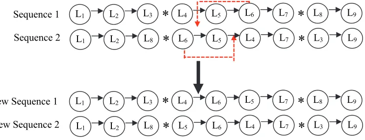
In the proposed GA, the chromosome is represented by each job and thus a schedule consists of (n+m−1) genes, denoted as 1 to n digits and (m−1) “∗” for separating the machines. By this means, the entire set of trains or trucks can be encoded on a single string in a Route/Rail Siding order. An example to depict this definition is provided in Fig. 4. Three sidings will be served by nine locomotives in the systems. The initial schedule of locomotives on each siding represents the chromosome or solution. The final schedule of locomotives is L1-L2-L3-L4-L5-L6-L7-L8-L9.
Fig. 4. Chromosome encoding (Sequence of locos or trucks on sidings)
4.2. Initial solution generation procedure
To generate random solutions for the initial population, the procedure is as follows: 1. Select trip 1; ∈ 1,2,3 … ,
2. Generate (B−1) asterisks “∗” and randomly assign to genes of the chromosome in which none of them are assigned to the first and the last genes, and between the asterisks there must be at least one unfilled gene. The total number of chromosomes is (P+B-2).
3. Assign the numbers from 1 to P to the rest of the unfilled genes of the chromosome.
4. Calculate the objective functions Ci values by using Constraint (1) and considering Constraint (2).
5. Check the precedence constraints; if the chromosome does not satisfy these constraints then go to Step 2 for replenishing the new chromosome.
6. Set p=p+1. If i > pop-size STOP, otherwise go to Step 2.
Pop size is the population size or the number of chromosomes at each population that is known in advance (Lipowski et al., 2012 p2193-2196). As a result, the fitness function of chromosomes for the first phase (i.e., the minimization of the train/truck total operating time) is defined as Eq. (1) and minimizes the total waiting in Eq. (2).
λ λ (2)
Siding 1
1
L L2 L3
*
L4 L5 L6 L7*
L8 L91
L L2 L3
4
L L5 L6 L7
8
L L9
R. Matindi et al.
λ λ (3)
(4)
As in Section 3.4, after applying the proposed GA to the first phase, the best fitness found for the first phase is added to the second phase as a constraint (i.e., the minimization of the total waiting time of harvesters and mill must be satisfied), where the proposed GA considers this constraint. The fitness function of the chromosomes for this phase is computed by Eq. (2).
4.3. Design of genetic operators
4.3.1. Patching crossover operator
Patching crossover operator is based on the crossover operator used in called a uniform order-based crossover. The algorithmic structure of this crossover is as follows:
1. Randomly choose two parents, Parent 1 (trip 1) and Parent 2 (trip 2), from the population. 2. Copy the genes from Parent 1 corresponding to the same positions in the child.
3. Cross out the genes from Parent 2 copied from Parent 1 so that the repetition of a gene in the new offspring is avoided.
4. Fill out the remaining empty gene locations with the uncrossed genes that remain in the parent by preserving their gene sequence in Parent 2.
5. Calculate Ci values by using Constraints (1) and (2).
6. Check the precedence constraints, if the chromosome does not satisfy these constraints then swap the place of the jobs that prevent the satisfaction of the precedence constraints.
4.3.2. Shift mutation operator
The main task of the mutation operator is to maintain the diversity of the population in the successive generation and to exploit the solution space. In this research, a mutation operator, called Shift Mutation, consists of shifting any two randomly chosen genes in a chromosome. At first, we define “mutation strength” as a demonstrator of maximum number of shift moves performed. If the strength of the mutation is chosen to be one, then it performs a single shift move, provided a given probability, namely P (M). So the strength of the mutation shows the number of consecutive shifts on the individual chromosome. In this paper, the mutation strength is set to two as follows in Fig. 5:
Fig. 5. Shifting mutation operator
Sequence 1 Sequence 2
*
*
1
L L2 L3 L4 L5 L6 L7 L8 L9
*
*
1
L L2 L8 L6 L5 L4 L7 L3 L9
New Sequence 1 New Sequence 2
*
*
1
L L2 L3 L4 L6 L5 L7 L8 L9
*
*
1
4.4. Parent selection strategy
The parent selection is important in regulating the bias in the reproduction process. The parent selection strategy relates to choosing chromosomes in the current population that will create offspring for the next generation. Generally, it is better that the best solutions in the current generation have more chance to be selected as parents in order to create offspring. The most common method for the selection mechanism is the “roulette wheel” sampling, in which each chromosome is assigned a slice of a circular roulette wheel and the size of the slice is proportional to the chromosome's fitness. The wheel is spun Pop Size times. On each spin, the chromosome under the wheel's marker is selected to be in the pool of parents for the next generation.
4.5. Offspring acceptance strategy
We use a semi-greedy strategy to accept the offspring generated by genetic operators. In this strategy, an offspring is accepted for the new generation if its fitness is less than the average fitness of its parent(s). This strategy reduces the computational time of the algorithm and leads to a monotonous convergence toward the optimum solution neighborhood.
4.6. Stopping rules
We use two criteria for stopping rules: (1) maximum number of an elapsed generation (Gmax) which is the relevant criterion and (2) standard deviation of the fitness value of chromosomes in the current generation. This parameter indicates a degree of diversity or similarity in the current population in terms of the objective function value (OFV). If the criterion stays lower than an arbitrary constant, the algorithm is terminated. The standard deviation of the fitness value of chromosomes in generation is computed using standard technique for standard deviation.
5. Analysing Production costs components
This section briefly discusses the main costs involved in the biomass recovery using the whole of cane harvesting with factory separation. In this section a highlight of how various costs were modelled as an exemplar is discussed (cane separation plant). The key changes that occur when the whole of cane recovery of biomass is adopted, is the installation of a separation plant, whose costs are discussed in the succeeding section.
5.1.1 Cane separator
The cost of cane separator was estimated using power factor applied to Plant capacity ratio.
In this method, the order of magnitude estimates the related fixed capital investment of a new process plant to the fixed capital investment of similar previously constructed plant. An exponent of 0.6 has been applied as documented by Peters et al. (1968) using the following relationship,
,
where is the cost index ratio at the time of cost to that at time .
5.1.2 Capital cost for Biorefinery operations– factory cane separation
R. Matindi et al.
∨
∀ ∈ , ∀ ∈ (5)
From Eq. (5), it can be deduced from the preceding disjunction that the linearized piece approximation equation to determine the capital cost for the cane separator depends on the size. The trigger point for the disjunctive function is ( Boolean variable for disjunction selection). In order to simulate the preceding disjunction, the convex hull technique is used (Ponce-Ortega et al., 2008 p5512; Gregg & Smith, 2010 p241), to obtain the following. The following constraints are postulated. The selection of disjunctive term can only be done per segment (i.e. one at a time).
1. ∀ ∈ (6)
The continuous variables are disaggregated for each domain of the disjunction , first for the pour rates (total sum of cane delivered and cleaned at the separation plant), is the harvester pour rate within linearized segments.
. ∀ ∈ (7)
The Total investment costs for cane separation plant are divided into capital cost and operating costs. However, commercially tested cane separators are constrained by maximum capacity, and in this case is 150 tonnes/h, for modelling purposes when this maximum capacity is reached, an additional unit is installed, Eq. (8) therefore models an aggregate of separation units needed to clean cane in a given set up.
,
, ∀ ∈ (8)
Then, the domain (limits) inside the disjunctions are reported in terms of the disaggregated variables.
∀ ∈ , ∀ ∈ (9)
∀ ∈ , ∀ ∈ (10)
The lower and upper limits are factored in the disaggregated variables as shown below
, ∀ ∈ , ∀ ∈ (11)
Non-negativity constraints
0, ∀ ∈ , ∀ ∈ (12)
where
Linearized domain minimum
Selection variable for domain determination Pour rate in linearized domain
Linearized domain maximum Cane Separation plant capital cost Maximum cost of Cane Separation plant
Cane Separator operation and maintenance cost for bioenergy product j Cane Separator operation and maintenance cost for bioenergy product k Cane Separator operation and maintenance cost for bioenergy product h Aggregate of whole of cane delivered
Aggregate of bioproducts H produced Aggregate of bioproducts K produced
Disjunction index of cane separator plant capital costs Location to set up the cane separation plant
Proportionality constant
The lower limits of the cane separator was obtained from the pilot Condong plant, while the upper limit were obtained the ongoing work of SRI study that is approximately 8 times the size of the pilot plant.
5.1.3 Operating costs
The key items considered to be operating costs for the separation plant include labor requirements and costs, utility or feedstock requirements, insurance costs and property taxes. The various subcomponents are all summed up, and the yearly O&M (Operation and Maintenance costs) are passed to the economic calculation table for inclusion in the final techno-economic component of the biorefinery cost. The relationship for the operating cost is therefore summarized as shown in equation below.
(14)
It is assumed that the above referenced costs are directly proportional to production volumes/size. Thus to analyse the net returns as the plant capacity increases and in effect the capital cost, sensitivity analysis was conducted on the three industry sectors, that is the Biomass producer net returns, the factory and by extension the biorefinery, and the overall effect to the industry. The lower bound represented the base case scenario (pilot plant in Condong) with its equivalent costs, while the upper case corresponds to the SRI pilot plant with an approximate size of eight times the base plant, the mid-sized cane cleaner was represented by the 5.5 Million dollars cane cleaning plant in Brazil. The cleaning plant efficiency ranges from 50- 95 %, at the following plant scale and cleaning efficiency and the following was found to be factory net returns.
R. Matindi et al.
6. Experimental results
6.1.2 Modelling factory, cogeneration plant performance for different levels of trash
The factory component of the integrated bioenergy system was modelled using pioneer mill and Broadwater mill entailed using propertiary SRI data and factory model to simulate site specific, sugar, molasses and power production and their associated costs. The approach adopted in this section was to simulate the factory production process as a function of mill throughput and cane quality, this in effect allowed the determination of trash impact on various section of the mill, and its implication in terms of cost. The factory components impacted by trash are the crushing plant, sugar extraction, molasses and sugar recovery, the cane feeding (cane tippler), low grade recovery of sugar and molasses, factory cane separator and cogeneration.
Having set the developed and the simulated with appropriate input data, the prediction capability of the system was validated against factory productivity/ mills reference records. The comparision between the factory data and predicted product streams (sugar , molasses and power are stipulated below),
And as indicated they are in good agreement with previous study (Hobson & Ridge, 2000).
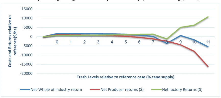
Fig. 6. The effect on Industry sector returns of changing levels of trash in the cane supply Fig. 6 typically simulates the varying trash levels on the various industrial sectors in sugar industry, which is composed of : the biomass producers, which represents sugarcane growers, the factory (which represent the mill), and the overall effect on the whole of industry. It can be deduced from the trend depicted above that, as trash levels increases in the supply, there is a drop for two sectors (i.e The whole of industry, and the net producer returns), this can be attributed to the fall in quality of the cane getting processsed, as CCS formula penalises extra introduction of trash in the system. There is an upshot in the factory sector returns, this being attributed to the extras biomass fibre being processed for bioenergy production purposes, thus for the factory to breakeven, more biomass is needed so that the capital cost could be be amortised over a wider fibre footprint.
6.1.2 Harvester cane Loss
The level of extraneous matter available in the cane supply are a direct function of the cleaning capability of the harvester. There are numerous sources that can occasion cane loss during harvesting, loading-up losses, extractor loss, basecutter loss and chopper loss, but the one with the biggest significant implication and in effect financial implications is the cleaning costs. Some of the key factors (production factors) affecting cane loss and under investigation in this study are: pour rate, extractor fan speeds, group sizes and crop conditions among other factors. Pour rate, Extractor fan speeds and and Trash levels in cane supply are taken as control factors or signal factors in this study, while the crop condition, yield and
‐20000
‐15000
‐10000
‐5000
0 5000 10000 15000
0 1 2 3 4 5 6 7 8 9 10 11
Co
st
s
an
d
Re
tu
rn
s
re
lative
ro
re
fe
ren
ce
($/ha)
Trash Levels relative to reference case (% cane supply)
group sizes are taken as noise factors. Harvesters are inherently deficient in terms of capability needed to balance the high pour rates and high cleaning fan speeds needed to ensure that both cane are clean and there is minimal loss. While there have been progress in terms of machine capaicity i.e. improved pour rates, cleaning system design is still lagging behind. As a result, considerable amount of loss of millable billets extracted by the cleaning system can be extreme, leading to huge losses to the industry. Thus, in order to assess the producers returns affected by cane loss. Fig. 7 shows the results of simulated scenarios to assess the impact of varying harvester fan speed and in effect cane loss, on the industry returns where trash levels are held constant. In order to hold the trash levels constant, harvester pour rates were adjusted and simulation ran for various rates. As shown in Fig. 6, as cane loss increases (i.e higher fan speeds), the net returns for all sectors of the industry decreases. Thus in absolute terms, the losses and gains associated with cane loss are more for the biomass producer due to the distribution of income from the sales of raw sugar.
Fig. 7. Effect of changes of relative cane loss on industry sector relative return ($/ha)
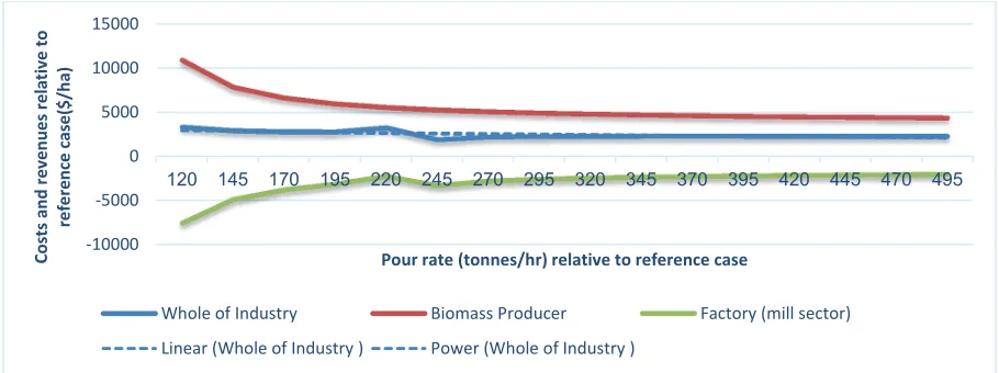
The effect of increasing pour rate on industry returns is stipulated in Fig. 7. It is deduced that, there was an overall decrease in the whole industry and biomass producer sectors in net returns when the harvester was operated between 120 tonnes/h and 220 tonnes/h, but the benefits, plateaus at at 250 tonnes/ha, implying the saturation point, in terms of benefits that could be accrued from increased pour rates. These simulated results concurred with previous study undertaken in different mill region in the within the Australia (Hobson, 2000).
Fig. 8 . Effect of Changes of relative Pour rate on industry sector relative return ($/ha)
Maximising industry sector return on “As is Scenario”
Two important levers within the harvesters that can drive the industry to profitability are pour rate and primary extractor fan speed (Hobson, 2000; Hobson et al., 2006). The two levers dictate the optimum
0 500 1000 1500 2000 2500 3000 3500 4000
4 5 6 7 8 9 10 11 12 13 14 15 16 17 18 19
Co st s an d re ven u e relative RTR C ($/h a)
Cane Loss relative to reference case (% cane supply)
Whole Industry return Biomass Producer Factory
‐10000 ‐5000 0 5000 10000 15000
120 145 170 195 220 245 270 295 320 345 370 395 420 445 470 495
Costs and revenues relative to re fe ren ce case ($/h a)
Pour rate (tonnes/hr) relative to reference case
Whole of Industry Biomass Producer Factory (mill sector)
R. Matindi et al.
amounts of trash that can be recovered, and the amount of cane loss that the industry can let go of. The fan speed has big effect on the cane loss and this effect has been included in the model. The simulation values for the referenced parameters were dictated by the latest harvester design and mill data availed.
6.1.1 Parameter Tuning using Taguchi Method
Taguchi method was employed at this stage to tune the production parameters under study, as it aids in improving consistency of production process and its robustness in the recognition that, not all factors that causes variability can be controlled. Thus Taguchi design inherently tries to identify controllable factors that minimises the effect of the noise factors. During the experimentation process, control factors were manipulated in order to evaluate variability that could occur, and to further, to determine the optimal control factor settings that minimises the process variability, this consequently yielded a robust design, that is able to output consistent results and performance regardless of the environment it is being used. In this study, a higher ratio of Signal to Noise design was being sought, this was done using a commercial statistical/industrial engineering software – Minitab, where factors were set at various levels (high and low). The factors of production selected for analyses that influence the overall industry returns are listed as; Pour rate, fan speed, and Trash levels (production factors being investigated). The levels of assessment for this study was set at two i.e. (high and low). The number of runs selected were 9, based on the design factors. The Noise in this scenario were related to crop conditions i.e. (Erect, or Not erect), Green or Burnt, overall Yield (High or Low), and the regional weather conditions characterising the area (Wet or Dry). The signal factors (production factors) that could improve the whole of industry returns were analysed using Taguchi design, using the experimental data obtained from the simulation work and pilot study. The following observations are made as stipulated in the following diagrams:
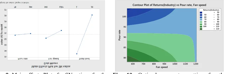
The signal to noise ratio (S/N ratio), for different levels of each production factor, are assessed. For production factor (pour rate), the Signal to noise ratio is highest, at the lower scale (78 t/h), i.e. level 1, while for fan speed, the Signal to Noise ratio is highest at level 1 (i.e. 543 rpm), while for trash level, Signal to noise ratio is highest at level 1.
Fig. 9. Main effects Plots for SN rations for the
production factors Fig. 10. Optimal parameter setting for the production factor that yield maximum returns Therefore, the optimal production with maximum consistency and returns is achieved where, factor (pour rate operates at level 1), fan speed and Trash are set at level 1. From the data, the highest signal to Noise ratio achieved correspond to the highest net industry returns, achieved as shown in Fig. 10. From this study, as shown in Fig. 10, the optimal settings that offers maximum returns to the industry is when in the production factor; fan speed is below 700 rpm, and pour rate at 78 t/h and hese settings are based on the harvester used in the study accomplished by Hobson and Ridge (2000). The experimental results confirm the findings from Hobson and Ridge (2000), who opined that based on harvester in their pilot study, the harvester settings that offered the maximum returns to the whole industry in Australia, was when pour rate was set at a lower scale (78 t/h), fan speed at 543 rpm and trash levels slightly above 1 % in the cane supply. This tuning process was repeated for all production factors evaluated in this study.
Fan speed
Po
ur
r
at
e
1200 1100 1000 900 800 700 600 100
95
90
85
80
> – – – – – – < 50
50 60
60 70
70 80
80 90
90 100
100 110
110 Returns(Industry)
6.1.2 Technology Assessment and Selection
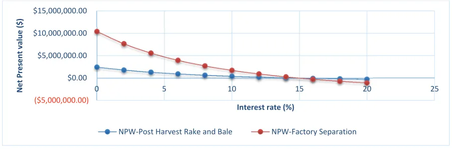
In order to evaluate the net present worth and in effect the preferred biomass recovery technique, the present benefits and the present costs were determined. Incremental analysis of the both alternatives was undertaken, after Rake and Bale and Whole of cane harvesting with factory recovery of trash showed positive returns based on various delivery cost, the incremental analysis was to sieve out the better option among the two recovery technology. In order to select an optimal recovery technique, incremental internal rate of return ∆ ) was computed. The rule of thumb while evaluating technology alternatives is that, for projects with positive IRR and with (∆ , the higher cost are chosen first, but where ∆ the lower costs are chosen first. Thus using the referenced rule, in this scenario, the whole crop harvesting and recovery (with factory separation of trash ) were found to offer higher returns. Fig. 11 shows that, the Net present worth between post recovery of biomass using rake and bale process, and the whole cane harvesting with factory separation of trash, for projects under 15 % interest rate, the net present value is higher for the factory separation in comparison with rake and bale, the point where the two line crosses, is the autarky point, where the benefits equals the costs.
Fig. 11. Net Present Worth - cane factory separation and Rake and Bale Process
Therefore for the recovery technique to remain and be deemed viable, all strategies employed must be evalauted on the positive side of the graph. Beyond the 15 % mark the net present value of whole of cane supply becomes unfavourable, as the net returns gets negative. However for the rake and bale, the recovery technology can still break even even at rates beyond the 15 % mark, i.e the net present value is constant at zero, which implies that the cost of recovery equals the accrued benefits.
6.1.3 Assessment of energy densification technique with Whole of cane harvesting and factory separation of trash
Fig. 12 shows the Net present worth between the post recovery of biomass using factory separation, Rake and bale process, Pelletisation, and TOP as a densification technology, and from the analysis it can be deduced that, the technology offering higher present returns is factory separation of trash. A comparison of the above scenario still has the factory separation as the process that gives the highest returns of approximately $ 11 millions. Beyond the 15 % mark only rake and bale technology is recommended as it plateaus at 15-20 % ranges. Factory separation of the whole cane, for projects under 15 % interest rate, the net present value is higher for the factory separation in comparison with rake and bale, where the two line crosses, is where the incremental analysis kicks in, and the benefits equals the costs, thus for a recovery method to be deemed sustainable and profitable all the interest rates must be evaluated on the positive side of the graph. Beyond the 15 % mark the net present value of the whole cane supply becomes unfavourable as the net returns gets negative. However for the rake and bale, the project can still be able to break even, i.e. the net present value is constant at zero, and that implies that the cost of recovery equals the accrued benefits. In order to evaluate the net present worth of the above referenced ventures, the present benefits and present costs, an incremental analysis of the alternatives was undertaken, after both rake and bale and the whole of cane harvesting with factory separation showed returns based on
($5,000,000.00)
$0.00 $5,000,000.00 $10,000,000.00 $15,000,000.00
0 5 10 15 20 25
Ne
t
P
res
ent
value
($)
Interest rate (%)
R. Matindi et al.
the various biomass delivery cost. They both exceeded the minimum rate of return, thus incremental analysis was performed to the two ventures to evaluate the better option. This was done using incremental internal rate of return ∆ , where if (∆ , the higher first cost was chosen, and if ∆
the economic rule is to choose lower first cost, so in this scenario, the whole of crop harvesting and recovery (Factory separation ) was found to offer higher returns.
Fig. 12. Net Present Worth (NPW) - Cane factory separation, Rake and Bale Recovery, Pelletisation and TOP Energy Densification Technology
7. Conclusion
There are a large numbers of attributes, parameters and resources, which make it almost impossible to model and establish enough mathematical relations to describe the processes. Besides, the time domain required to model and run every event has a stochastic distribution, which leaves uncertainty in the exactitude of the processes output. However, simulation modelling is able to mimic every process of production, and thus presents an alternative technique to mathematical programming. The application of the simulation model for the sizing of the recovery equipment requires large amount of data mostly from the mills and biomass producer, pilot plants (i.e. modelling the separation processes) among others. The developed tool bioenergy tool has simulated the harvesting, infield transportation, main transportation, bagasse production, storage and power production. The whole of cane recovery process with factory separation has been demonstrated to be the cheapest recovery technique, besides offering high net present return relative to a reference plant, amongst all technologies evaluated. Further, all the energy densification techniques have been shown to break even at the prevailing hurdle rate of at least 10 %. In evaluating the alternative bioprocesses of energy densification, it has been established that strategies adopting factory separation as a precursor recovery technique for the feedstock has the highest net present worth relative to a reference case. It has further been established that, in order to fully optimise a bioenergy system, resource management plays a significant role, and proper utilisation of the same besides proper settings can drive the bioenergy sector to profitability. A scheduling regime was modelled for the case study under investigation, while its direct net benefits in terms of cost, may not be apparent or quantified in this study, the new scheduling algorithm can be patched to the existing schedules to optimise the operations of a biorefinery as envisaged in the conceptual study above.
References
Asikainen, A., Liiri, H., Peltola, S., Karjalainen, T., & Laitila, J. (2008). Forest energy potential in Europe (EU27). Finnish Forest Research Institute, Vantaa.
Bowling, I. M., Ponce-Ortega, J. M., & El-Halwagi, M. M. (2011). Facility location and supply chain optimization for a biorefinery. Industrial & Engineering Chemistry Research, 50(10), 6276-6286.
Brinsmead, T. S., Herr, A., & O'Connell, D. A. (2015). Quantifying spatial dependencies, trade‐offs and uncertainty in bioenergy costs: An Australian case study (1)–least cost production scale. Biofuels, Bioproducts and Biorefining, 9(1), 21-34.
($5,000,000.00)
$0.00 $5,000,000.00 $10,000,000.00 $15,000,000.00
0 5 10 15 20 25
Ne
t
P
res
ent
Value
($)
Interest rate (%)
Dias, M. O., Junqueira, T. L., Cavalett, O., Cunha, M. P., Jesus, C. D., Rossell, C. E., ... & Bonomi, A. (2012). Integrated versus stand-alone second generation ethanol production from sugarcane bagasse and trash. Bioresource technology, 103(1), 152-161.
Farine, D. R., O'Connell, D. A., John Raison, R., May, B. M., O'Connor, M. H., Crawford, D. F., ... & Dunlop, M. I. (2012). An assessment of biomass for bioelectricity and biofuel, and for greenhouse gas emission reduction in Australia. GCB Bioenergy, 4(2), 148-175.
Gan, J., & Smith, C. T. (2006). A comparative analysis of woody biomass and coal for electricity generation under various CO 2 emission reductions and taxes. Biomass and Bioenergy, 30(4), 296-303.
Gregg, J. S., & Smith, S. J. (2010). Global and regional potential for bioenergy from agricultural and forestry residue biomass. Mitigation and Adaptation Strategies for Global Change, 15(3), 241-262.
Hobson, P. A., & Ridge, D. R. (2000). SRDC project BS157S: Analysis of field and factory options for efficient gathering and utilization of trash from green cane harvesting.
Hobson, P. A., Edye, L. A., Lavarack, B., & Rainey, T. J. (2006). Analysis Of Bagasse And Trash Utilization Options-SRDC Technical Report 2/2006.
Ikonen, T., Asikainen, A., Prinz, R., Stupak, I., & Smith, T. (2013). Economic sustainability of biomass feedstock supply. IEA Bioenergy Task 43: 2013: 01. Technical report.
Lipowski, A., & Lipowska, D. (2012). Roulette-wheel selection via stochastic acceptance. Physica A: Statistical Mechanics and its Applications, 391(6), 2193-2196.
Masoud, M., Kozan, E., & Kent, G. (2015). Hybrid metaheuristic techniques for optimising sugarcane rail operations. International Journal of Production Research, 53(9), 2569-2589.
Masoud, M., Kozan, E., Kent, G., & Liu, S. Q. (2016). An integrated approach to optimise sugarcane rail operations. Computers & Industrial Engineering, 98, 211-220.
Meyer, J. C., Hobson, P. A., & Schultmann, F. (2012). The potential for centralised second generation hydrocarbons and ethanol production in the Australian sugar industry. In Proceedings of the Australian Society of Sugar Cane Technologists (Vol. 34).
Peters, M. S., Timmerhaus, K. D., West, R. E., Timmerhaus, K., & West, R. (1968). Plant design and economics for chemical engineers (Vol. 4). New York: McGraw-Hill.
Ponce-Ortega, J. M., Jiménez-Gutiérrez, A., & Grossmann, I. E. (2008). Simultaneous retrofit and heat integration of chemical processes. Industrial & Engineering Chemistry Research, 47(15), 5512-5528.
Resch, G., Held, A., Faber, T., Panzer, C., Toro, F., & Haas, R. (2008). Potentials and prospects for renewable energies at global scale. Energy Policy, 36(11), 4048-4056.
Ranta, T., Korpinen, O. J., Jäppinen, E., & Karttunen, K. (2012). Forest biomass availability analysis and large-scale supply options. Open Journal of Forestry, 2(1), 33.
Raulund-Rasmussen, K., Stupak, I., Clarke, N., Callesen, I., Helmisaari, H. S., Karltun, E., & Varnagiryte-Kabasinskiene, I. (2008). Effects of very intensive forest biomass harvesting on short and long term site productivity. In Sustainable use of forest biomass for energy (pp. 29-78). Springer Netherlands.
Rivers, N., & Jaccard, M. (2005). Canada's efforts towards greenhouse gas emission reduction: a case study on the limits of voluntary action and subsidies. International Journal of Global Energy Issues, 23(4), 307-323. Sims, R. E., Mabee, W., Saddler, J. N., & Taylor, M. (2010). An overview of second generation biofuel
technologies. Bioresource technology, 101(6), 1570-1580.
Sundarakani, B., De Souza, R., Goh, M., Wagner, S. M., & Manikandan, S. (2010). Modeling carbon footprints across the supply chain. International Journal of Production Economics, 128(1), 43-50.
Thorburn, P. J., Archer, A. A., Hobson, P. A., Higgins, A. J., Sandell, G. R., Prestwidge, D. B., ... & Juffs, R. (2006). Value chain analyses of whole crop harvesting to maximise co-generation. In PROCEEDINGS-AUSTRALIAN SOCIETY OF SUGAR CANE TECHNOLOGISTS (Vol. 2006, p. 37).
Thorburn, P. J., Sandel, G. R., Antony, G., Juffs, R., Archer, A. A., Hobson, P. A., ... & Higgins, A. J. (2005). Integrated value chain scenarios for enhanced mill region profitability.
Thorburn, P. J., Archer, A. A., Hobson, P. A., Higgins, A. J., Sandel, G. R., Prestwidge, D. B., & Antony, G. (2007). Evaluating regional net benefits of whole crop harvesting to maximise co-generation. In Proc. Int. Soc. Sugar Cane Technol (Vol. 26).