www.atmos-meas-tech.net/9/587/2016/ doi:10.5194/amt-9-587-2016
© Author(s) 2016. CC Attribution 3.0 License.
A total sky cloud detection method using real clear sky background
Jun Yang1,2, Qilong Min2,3, Weitao Lu1, Ying Ma1, Wen Yao1, Tianshu Lu1, Juan Du3, and Guangyi Liu4 1State Key Laboratory of Severe Weather, Chinese Academy of Meteorological Sciences, Beijing 100081, China 2Atmospheric Sciences Research Center, State University of New York, Albany, NY 12203, USA
3School of Remote Sensing and Information Engineering, Wuhan University, Wuhan 430079, China 4Smart Grid Operation Research Center, China Electric Power Research Institute, Beijing 100192, China
Correspondence to: Q. Min ([email protected])
Received: 6 November 2015 – Published in Atmos. Meas. Tech. Discuss.: 10 December 2015 Revised: 6 February 2016 – Accepted: 9 February 2016 – Published: 23 February 2016
Abstract. The brightness distribution of sky background is usually non-uniform, which creates many problems for tradi-tional cloud detection methods, including the failure of thin cloud detection in total sky images and significantly reduc-ing retrieval accuracy in the circumsolar and near-horizon re-gions. This paper describes the development of a new cloud detection algorithm, named “clear sky background differ-encing (CSBD)”, which is accomplished by differdiffer-encing the original image and the corresponding clear sky background image using the images’ green channel. First, a library of clear sky background images with a variety of solar eleva-tion angles needs to be developed. The image rotaeleva-tion and image brightness adjustment algorithms are applied to en-sure the two images being differenced have the same solar position and similar brightness distribution. Sensitivity tests show that the cloud detection results are satisfactory when the two images have the same solar positions. Several exper-imental cases show that the CSBD algorithm obtains good cloud recognition results visually, especially for thin clouds.
1 Introduction
Clouds are an essential part of the atmospheric energy and water cycle, and their coverage state is crucial for radiative transfer models and climate simulations. Traditional visual observations have been carried out worldwide at meteoro-logical stations to estimate sky cloud amount for more than 100 years (Deutscher Wetterdienst, 2013). So far, human ob-servations are still the main means of obtaining surface cloud coverage in many countries. However, the subjectivity of vi-sual observations introduces significant uncertainty into the
accuracy of cloud coverage measurement. In the Automated Surface Observing System program, a laser ceilometer is widely used, instead of visual observations, to retrieve whole sky cloud amount based on a time series of ceilometer data. The more direct means of determining cloud cover is using a digital camera and a fisheye lens to capture total sky visible images and adopting a certain cloud detection algorithm to calculate cloud coverage. A number of such instruments have been reported in the literature, such as the Whole-Sky Imager (WSI, Shields et al., 1993), the Whole-Sky Camera (WSC, Calbó and Sabburg, 2008; Long et al., 2006), the All-Sky Imager (Huo and Lu, 2009; Cazorla et al., 2008), the Total-sky Cloud Imager (TCI, Yang et al., 2012), the Automatic-capturing Digital Fisheye Camera (ADFC, Yamashita and Yoshimura, 2012), the All Sky Infrared Visible Analyzer (ASIVA, Klebe et al., 2014), and the PROMES-CNRS sky imager (Chauvin et al., 2015). The Total Sky Imager (TSI, Long and Deluisi, 1998) is a commercial instrument used to capture total sky images using a charge-coupled device look-ing downward onto a parabolic mirror. The strong forward scattering of the sun greatly impedes the ability of the digi-tal camera to acquire a good todigi-tal sky image. Most of these imagers adopt a solar tracking shadowband to occlude the in-tense direct solar radiation, while others, such as TCI, ADFC, and ASIVA, use auto exposure (AE) technologies, instead of a sun shielding device, to retrieve a satisfying total sky im-age.
detec-tion algorithms have been implemented on the aforemen-tioned devices using these properties. The methods adopt-ing the blue (B) and the red (R) channels to separate cloud pixels from the sky background have been used by many researchers. Koehler et al. (1991) discriminated between opaque cloud, thin cloud, and clear sky by defining two thresholds in the R/B ratio space for the WSI images. Long et al. (2006) recommend a single threshold of 0.6 to clas-sify the cloudy pixels, also in the R/B space, but for the WSC images instead. The differencing of R−B replaced the R / B ratio in the method of Heinle et al. (2010), in which they suggested R−B=30 as a better threshold for cloud identification. The fixed threshold (FT) algorithms ob-tained satisfactory detection results for opaque clouds but of-ten failed for thin clouds and encountered some issues in the circumsolar region. The brightness distribution of ferent total sky images changes significantly because of dif-ferent imaging instruments and illumination conditions, pre-venting the application of FT methods to all images. Li et al. (2011) proposed a hybrid threshold algorithm to estimate clouds in the (R−B)/(R+B) color space. Yang et al. (2012) put forward the background subtraction adaptive threshold algorithm to segment clouds in the same (R−B)/(R+B) color space. In addition to these 2-D red and blue channel algorithms, several methods have been developed to detect clouds based on the 3-D red-green-blue (RGB) color space. Sylvio et al. (2010) considered all RGB information in or-der to accurately detect clouds, and their algorithm combined both Bayesian statistics and Euclidean geometric distance. Kazantzidis et al. (2012) followed the idea of R−B differ-ence and proposed a multicolor criterion to identify cloudy pixels from the no-sun-shadowing whole-sky images. Ya-mashita and Yoshimura (2012) defined sky index (SI) and brightness index (BI) in the RGB color space for the whole-sky images and classified the sun, blue whole-sky, and clouds using the threshold curve developed from 2-D BI and SI coordi-nates. Souza-Echer et al. (2006) transferred the images from the RGB color space to the hue saturation intensity space and presented a cloud detection method only using 1-D sat-uration information. Most existing cloud identification algo-rithms encounter great uncertainties for cloud detection in the circumsolar and near-horizon regions. To face this challenge, Long et al. (2006) established a clear-sky function to identify clear, thin, and opaque clouds for the TSI images, and then Long (2010) proposed a statistical analysis method to correct the cloud identification errors in those regions. The technol-ogy operates by simulating clear sky background (CSB) and by computing the difference with the original image to obtain improved cloud identification results. Ghonima et al. (2012) classified clear, opaque, and thin clouds from the TSI im-ages by utilizing red-blue ratio to subtract the clear sky li-brary, which is a function of image zenith angles, sun-pixel angle, and solar zenith angle. Chauvin et al. (2015) simulated clear sky background using least squares fitting in the nor-malized red/blue ratio space. All of these algorithms assume
the RGB information of the images is correct and reliable. However, by analyzing the imaging principle of the cameras, Yang et al. (2015) found, after using the Bayer color filter ar-ray (CFA, Bayer, 1976) and various demosaicing algorithms (Kimmel, 1999), that the RGB color images acquired from the cameras do not represent true color, and the channel’s operation will magnify this divergence from true represen-tation. Since the CFA filter adopts more green pixels than blue or red pixels, to simulate the human eye’s sensitivity to green light, Yang et al. (2015) suggested using a 1-D green channel instead of the 2-D red-to-blue or the 3-D RGB al-gorithms to perform cloud detection, especially for partly cloudy images. The green channel background subtraction adaptive threshold (GBSAT) method (Yang et al., 2015) sim-ulated background brightness of the green channel using a morphological operation and had better cloud identification accuracy than the traditional methods, especially in the cir-cumsolar and near-horizon regions. It is true that the sim-ulated background sometimes cannot characterize the true sky background; this will induce some detection errors, es-pecially for the thin clouds.
Accordingly, we put forward a new cloud detection algo-rithm, named “clear sky background differencing” (CSBD), which adopts a real clear sky background, rather than a simu-lation, to improve the cloud detection accuracy. The imaging device and image data are introduced in Sect. 2. Section 3 de-scribes the CSBD algorithm in detail. Several TCI images at different weather conditions are analyzed to verify the valid-ity of the proposed algorithm in Sect. 4. Finally, a summary and suggestions for future research are shown in Sect. 5.
2 Device and data
0 100 200
0.0 0.2 0.4 0.6 0.8 1.0 N o rm a liz e d fr re q u e n c y Brightness (a) (b) 23 46 (d)
Figure 1. Relationships between the exposure time and the
bright-ness value for the TCI images. (a) TCI image at exposure time of 300 µs, (b) TCI image with the same lighting conditions and camera parameters as in (a), but with 600 µs exposure time, (c) difference of 2×(a) and (b) for the green channel, and (d) normalized brightness
histograms distribution for the green channel of (a) and (b).
of Fig. 1a. Figure 1c, in which most of pixel values are zeros except for some pixels with non-zero noises, is the result of the difference of 2×(a) and (b) for the green channel. The normalized brightness histograms’ distribution and the green channel peaks of Fig. 1a and b are shown in Fig. 1d. The multiplicative relationship between the two peaks (their gray values are 23 and 46) can represent the exposure time differ-ence of the two images; although the lighting conditions and exposure time for any two TCI images vary, we can make the two images have very similar background brightness by ad-justing their gray histograms. This property will be used later in the algorithm analysis.
3 Cloud detection algorithm
In this section, we give an overview for the proposed CSBD algorithm, introduce how to set up the database of clear sky backgrounds, and describe the details of CSBD using an ex-ample. Finally, some sensitivity tests and limitations of the algorithm are presented.
3.1 Overview
Depending on the proportion of clouds in the sky, the sky type can be classified into clear, partly cloudy, and overcast. Li et al. (2011) and Yang et al. (2015) presented a method to distinguish sky type from total sky images using bright-ness histogram analysis. The radiometric data can be used to classify these three sky types accurately (Alonso et al.,
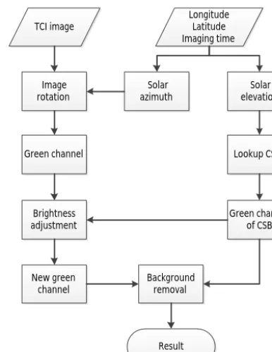
Green channel Solar azimuth Image rotation Lookup CSBL Green channel of CSB Brightness adjustment New green channel Background removal Result Solar elevation Longitude Latitude Imaging time TCI image
Figure 2. Flowchart of the proposed algorithm.
2014; Chu et al., 2014). Determining the cloud coverage of clear sky and overcast images is relatively easy because of their cloudless or all-sky cloud properties, so the pro-posed algorithm focuses mainly on partly cloudy images. All subsequent total sky images were obtained in Tibet, China, (88.88◦E, 29.25◦N) by a TCI device from 20 August 2012 to 5 July 2014. The CSBD algorithm first needs to build a clear sky background library (CSBL) for plenty of predefined solar elevation angles, which is accomplished by rotating the orig-inal TCI clear sky images with the angles equal to the solar azimuth. Then, for any cloud image of TCI, the longitude and latitude of TCI location and its imaging time will be used to calculate the solar azimuth angle and the solar elevation an-gle, and then its green channel is selected to perform cloud detection. Based on the solar elevation angle of the cloudy image, the corresponding CSB image, which will be used to perform differencing with the partly cloudy image, can be re-trieved in the CSBL. The detailed flowchart of the algorithm is shown in Fig. 2, which will be explained in the following subsections in detail.
3.2 Real clear sky background library
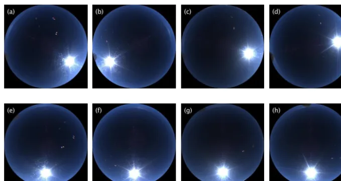
Figure 3. Several TCI images of different imaging times and the results after rotation. Panels (a) and (b) are the TCI images shot in the
morning and afternoon of 8 October 2012, image (c) is captured on 5 April 2013, (d) is obtained on 11 June 2013, with (e) through (h) as the corresponding rotation images of (a) to (d).
site. Many solar positioning algorithms have been developed to calculate the solar azimuth and solar elevation angle for a named time and a given longitude and latitude (Spencer, 1971; Michalsky, 1988; Meeus, 1998; Blanco-Muriel et al., 2001). The TCI images are typically oriented in a fashion such that north is up, south is down, west is left, and east is right. Based on the solar azimuth and solar elevation angle information, Yang et al. (2015) proposed a solution to deter-mine the position of the sun in the TCI images. For a fixed observation site, the positions of the sun in the images are hardly consistent for any two different imaging times. This is a big challenge for us to establish the CSBL. If we build the CSBL to include the CSB images for all times, the database will be too large and complex.
Fortunately, using the symmetry of the total sky images (Huo and Lu, 2009), we can rotate each TCI image along the center of the image and the center of the sun, where the rota-tion angle is equal to the solar azimuth. Figure 3a and b are two TCI images acquired in the morning and afternoon of 8 October 2012. Obviously, the positions of the sun in these two images are completely different, though they have the same solar elevation angles; one is on the right of the image, and the other is on the left. After image rotation, the centers of the sun in the two images (see the Fig. 3e and f) are almost completely coincident. Here, to better preserve the brightness information of the original images, the nearest-neighbor in-terpolation algorithm is adopted when performing image ro-tation. Another two TCI images (Fig. 3c and d) are captured at different dates. They also have the same solar elevation an-gles but different solar azimuth anan-gles, resulting in entirely different coordinates of the sun between the two images. Fig-ure 3g and h show the results after image rotation, in which the positions of two solar centers are exactly the same. Actu-ally, the four TCI images (Fig. 3a–d) have equal solar
eleva-tion angles. Using the technique of image rotaeleva-tion, the CSB for these four times in the CSBL can be represented using any one of Fig. 3e–h.
Every day the sun rises from the east and sets in the west, and the solar azimuth angle and the solar elevation angle change constantly. For any TCI image, by rotating the im-age with an angle equal to the solar azimuth, the sun will always be situated at the lower half of the perpendicular bi-sector of the image. The distance from the center of the sun to the center of the image is determined by the solar eleva-tion angle, so we build a database representing the real clear sky background with different solar elevation angles. The in-terval of the solar elevation angles in the CSBL is 1◦. Fig-ure 4 shows examples of the CSBL for some typical CSB images, which were captured on 11 June 2013. The CSBL is updated on every clear sky day through the year because aerosols and climate affect the brightness distribution of the clear sky. Therefore, when the proposed cloud detection al-gorithm is applied to a certain TCI image, the CSB image with the same solar elevation angle and the closest date as the TCI image will be selected to perform cloud detection.
3.3 Cloud detection method using real clear sky background
Figure 4. Several typical clear sky background images captured on 11 June 2013. The solar elevation angles of (a) to (h) range from 10 to
80◦at intervals of 10◦.
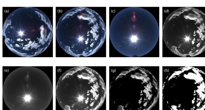
Figure 5. Cloud detection result based on CSB. Panel (a) is the original TCI image captured on 7 June 2013, (b) is the image after rotation, (c) is the real clear background image with the same solar elevation angle as (b), (d) shows the green channel of (b), (e) shows the green
channel of (c), (f) represents the new green channel of (d) after brightness adjustment, which has very similar brightness distribution to
(e) especially for sky background, (g) is the difference of (f) and (e), and (h) is the ultimate cloud detection result.
image. Then, the green channels of the images are separated from the RGB color images. By analyzing the brightness his-tograms of the green channels, the gray values of the cloudy image are adjusted, pixel by pixel, by multiplying or divid-ing by a number to ensure the two green channel images have the similar background brightness distribution. The number is determined by the ratio of the peak positions of the two histograms. Finally, the differencing and binarization meth-ods are applied to obtain the final cloud detection result.
Figure 5 shows an example to illustrate each step of the proposed CSBD algorithm. Figure 5a is the original TCI im-age acquired on 7 June 2013, and Fig. 5b represents the re-sulting image after image rotation. Figure 5c is the CSB im-age captured on 26 May 2013, which has the same solar
el-evation angle (68◦) as Fig. 5b. Figure 5d and e are the green
1
2
3
(a) (b) (c) (d) (e)
4
Figure 6. Sensitivity test for low solar elevation angle. (a) is the TCI image after rotation,
5
which was captured on 11 October 2012, (b) is the CSB images, where the first row has the
6
completely same solar elevation angle as (a), the solar elevation angle of the second row has
7
2 deviation with (a), and the solar elevation angle of the third row has 5 deviation with (a), (c)
8
is the difference images, (d) is the corresponding cloud detection results, (e) represents the
9
differencing results between the 2 and 5 offset with the baseline result in row 1.
10
11
Figure 6. Sensitivity test for low solar elevation angle. Panel (a) is the TCI image after rotation, which was captured on 11 October 2012,
column (b) shows the CSB images, where the first row has completely the same solar elevation angle as (a), the solar elevation angle of
the second row has 2◦deviation with (a), and the solar elevation angle of the third row has 5◦deviation with (a), (c) shows the difference
images, (d) shows the corresponding cloud detection results, and (e) represents the differencing results between the 2 and 5◦offset with the
baseline result in row one.
regions in the visual comparison. For some thin clouds, this method can also give an accurate identification. Even some bright noises, caused by the refraction of the light, are suc-cessfully excluded from the detection result because of their constant positions and similar brightness in Fig. 5e and f.
3.4 Sensitivity tests
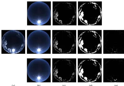
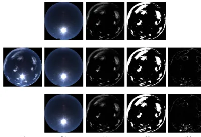
The theoretical basis of the proposed CSBD algorithm is that two images have similar brightness distribution as long as the positions of the sun in the images are the same; so a correct CSB image is critical for the accurate cloud detection. To check the influence of the CSB images with different solar elevation angles on our algorithm, we performed some sen-sitivity tests. Figure 6 shows the cloud detection results for a TCI image based on different CSB images. Figure 6a shows the original TCI image after rotation, which was taken on 11 October 2012, with its solar elevation angle equal to 33◦.
Figure 6b represents three different CSB images. Figure 6c shows the resulting difference images, and Fig. 6d shows the corresponding cloud detection results. The CSB image in the first row has completely the same solar elevation angle as Fig. 6a, while the solar elevation angle of the CSB image in the second row deviates 2◦from Fig. 6a, and the deviation of solar elevation angle in the last row is 5◦. It is obvious that
the cloud detection result in the first row is better than the others because the CSB image in that row has solar elevation angles identical to Fig. 6a. Figure 6e represents the differ-encing results between the 2 and 5◦offset with the baseline result in row one. When there is a deviation of solar elevation angle between the two images, some cloud detection errors will appear, especially in the circumsolar region. The greater the deviation angle, the greater the cloud detection errors.
1
2
3
(a) (b) (c) (d) (e)
4
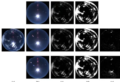
Figure 7. Sensitivity test as Fig. 6 but for medium solar elevation angle. (a) is the TCI image
5
after rotation, which was captured on 20 March 2013, (b) is the CSB images, where the first
6
row has the completely same solar elevation angle as (a), the solar elevation angle of the
7
second row has 2 deviation with (a), and the solar elevation angle of the third row has 5
8
deviation with (a), (c) is the difference images, (d) is the corresponding cloud detection
9
results, (e) represents the differencing results between the 2 and 5 offset with the baseline
10
result in row 1.
11
12
Figure 7. Sensitivity test as Fig. 6 but for medium solar elevation angle. Panel (a) is the TCI image after rotation, which was captured on
20 March 2013, (b) shows the CSB images, where the first row has the completely same solar elevation angle as (a), the solar elevation
angle of the second row has 2◦deviation with (a), and the solar elevation angle of the third row has 5◦deviation with (a), (c) shows the
difference images, (d) shows the corresponding cloud detection results, (e) represents the differencing results between the 2 and 5◦offset
with the baseline result in row one.
3.5 Limitations
The proposed CSBD algorithm is suitable for the detection of clouds in partly cloudy total sky images, especially when the sun is not obscured by clouds. However, if the sun is blocked by clouds partially or completely, the intensity of the Mie scattering is significantly weaker than the strength of the for-ward scattering of the sun, resulting in the failed detection result of the CSBD algorithm in the circumsolar region. The examples in the first row of Fig. 9 portray this limitation. Figure 9a is the original TCI image after rotation, which was obtained on 25 August 2012, Fig. 9b shows the CSB image retrieved in the CSBL, Fig. 9c presents the difference be-tween the two images (Fig. 9a and b), and Fig. 9d denotes the final cloud detection result. This limitation can be improved by combing the detection result in the circumsolar region. Yang et al. (2015) presented a method to determine the cen-ter coordinate of the sun, and by prescribing a radius around this coordinate, we can define the range of the circumsolar region. Setting a suitable threshold for the green channel, we can obtain the cloud pixels in the circumsolar region. Merg-ing these results, a more accurate cloud detection result can be obtained.
The second row of Fig. 9 shows the other limitation for the CSBD algorithm. The original TCI image was taken on
23 August 2012. When the clouds are optically thick and the cloud base height is very low, the brightness of these clouds is very low, sometimes even darker than the pixels in the CSB image; this phenomenon will inevitably introduce some de-tection errors for these pixels (see the left region in the sec-ond row of Fig. 9). Considering the traditional 2-D red-to-blue methods have very high detection accuracy for optically thick clouds, these two results can be merged to improve the identification accuracy of clouds.
4 Results comparison
al-1
2
3
(a) (b) (c) (d) (e)
4
Figure 8. Sensitivity test as Fig. 6 but for high solar elevation angle. (a) is the TCI image after
5
rotation, which was obtained on 28 June 2013, (b) is the CSB images, where the first row has
6
the completely same solar elevation angle as (a), the solar elevation angle of the second row
7
has 2 deviation with (a), and the solar elevation angle of the third row has 5 deviation with (a),
8
(c) is the difference images, (d) is the corresponding cloud detection results, (e) represents the
9
differencing results between the 2 and 5 offset with the baseline result in row 1.
10
11
Figure 8. Sensitivity test as Fig. 6 but for high solar elevation angle. Panel (a) is the TCI image after rotation, which was obtained on
28 June 2013, (b) shows the CSB images, where the first row has the completely same solar elevation angle as (a), the solar elevation angle
of the second row has 2◦deviation with (a), and the solar elevation angle of the third row has 5◦deviation with (a), (c) shows the difference
images, (d) shows the corresponding cloud detection results, and (e) represents the differencing results between the 2 and 5◦offset with the
baseline result in row one.
1
2
(a) (b) (c) (d)
3
Figure 9. The limitations of the proposed method. (a) is the TCI images after rotation, (b) is 4
the corresponding CSB images, (c) is the difference images, and (d) represents the final cloud 5
detection results. 6
7
Figure 9. The limitations of the proposed method. Column (a) shows the TCI images after rotation, (b) shows the corresponding CSB
images, (c) shows the difference images, and (d) represents the final cloud detection results.
gorithm. Of all these results, the white pixels represent cloud and black pixels are sky regions.
Quantitatively evaluating the precision of different cloud detection methods is considerably difficult because, if we
1
2
3
4
5
(a) (b) (c) (d) (e) 6
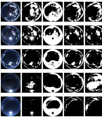
Figure 10. Comparison for different cloud detection methods. (a) is the TCI images after
7
rotation, (b) represents the results of R/B, (c) is the results of multi-color method, (d) denotes
8
the results of GBSAT, and (e) is the results of the proposed CSBD method.
9
Figure 10. Comparison of different cloud detection methods. Column (a) shows the TCI images after rotation, (b) represents the results
of R/B, (c) shows the results of multicolor method, (d) denotes the results of GBSAT, and (e) shows the results of the proposed CSBD method.
this comparison, we simply evaluate the precision of differ-ent cloud detection methods by visual examination. The re-sults of the 2-D R/B method are acceptable for some thick clouds but are unacceptable for the vast majority of thin clouds. When the sun is visible in the TCI images, the 2-D R/B method misclassifies most sun pixels into cloud pix-els. Of all these algorithms, the 3-D multicolor method incor-rectly identified most sky pixels as cloud pixels, especially in the circumsolar and near-horizon regions. The reason may be that some fixed multicolor criterions are not suitable for our TCI instruments and local climatic conditions. The GBSAT
5 Conclusions
The purpose of this paper was to introduce a new cloud detec-tion algorithm for the total sky partly cloudy images. Tradi-tionally, the 2-D R/B methods were widely used and accepted as standard algorithms to detect clouds. The 3-D RGB meth-ods were developed by some researchers in order to improve the accuracy of cloud detection. However, Yang et al. (2015) suggested using the 1-D green channel of the RGB image in-stead of the 2-D R/B and the 3-D RGB methods for cloud detection methods by analyzing the imaging principle of the color camera; so, in this paper, the proposed CSBD algorithm was based on the green channel of the images. The database of CSBL was built by rotating the original TCI images for clear sky conditions. The center of the sun was always on the perpendicular bisector of the image in the CSBL. For any single cloudy TCI image, the CSB image with the same so-lar elevation angle as the TCI image was retrieved from the CSBL. The histogram adjustment was performed to ensure the two images had similar brightness distribution. Finally, the differencing and binarization processing were applied to obtain the final cloud identification result. The test results showed that the proposed CSBD algorithm outperforms the traditional methods, especially in the circumsolar and near-horizon regions and for thin clouds when the sun is visible in the image. Additionally, some bright noises, due to the re-fraction of light, can also be correctly classified as non-cloud pixels.
It needs to be noted that the CSBD algorithm still has some limitations. When the overlying clouds are thick and the cloud base heights are low, the brightness values of these cloud pixels are even lower than the corresponding pixels in the CSB image. The single CSBD algorithm may misclas-sify these cloud pixels as clear pixels. The accurate thick cloud identification from the 2-D red-to-blue methods can be combined to improve the cloud detection accuracy of this new algorithm. Additionally, when the sun is obscured by clouds, partially or completely, the identification result may miss some cloud pixels in the circumsolar region. This limi-tation can be improved by merging the cloud detection result in the circumsolar region with the CSBD result.
Acknowledgements. This work was supported by the National
Key Scientific Instrument and Equipment Development Projects of China (grant 2012YQ11020504), the National Natural Science Foundation of China (grant 41105121 and grant 41105122), and the Basic Research Fund of Chinese Academy of Meteoro-logical Sciences (2015Y010). We also appreciate funding from the Science and Technology Research Foundation of SGCC, contract DZB17201200260. We are grateful to Emily Morgan for polishing the English grammar of the paper.
Edited by: A. Kokhanovsky
References
Alonso, J., Batlles, F. J., López, G., and Ternero, A.: Sky camera im-agery processing based on a sky classification using radiometric data, Energy, 68, 599–608, 2014.
Bayer, B. E.: Color imaging array, US patent 3971065, Alexandria, Virginia, USA, 10 pp., 1976.
Blanco-Muriel, M., Alarcon-Padilla, D. C., Lopea-Moratalla, T., and Lara-Coira, M.: Computing the solar vector, Sol. Energy, 70, 431–441, 2001.
Calbó, J. and Sabburg, J.: Feature extraction from whole-sky ground-based images for cloud-type recognition, J. Atmos. Ocean. Tech., 25, 3–14, 2008.
Cazorla, A., Olmo, F. J., and Alados-Arboledas, L.: Development of a sky imager for cloud cover assessment, J. Opt. Soc. Am. A., 25, 29–39, 2008.
Chauvin, R., Nou, J., Thil, S., Traoré, A., and Grieu, S.: Cloud detection methodology based on a sky-imaging system, Energy Procedia, 69, 1970–1980, 2015.
Chu, Y., Pedro, H. T. C., Nonnenmacher, L., Inman, R. H., Liao, Z., and Coimbra, C F. M.: A smart image-based cloud detection system for intrahour solar irradiance forecasts, J. Atmos. Ocean. Tech., 31, 1995–2007. 2014.
Deutscher Wetterdienst: German Climate Observing Systems. In-ventory report on the Global Climate Observing System (GCOS), self-published by DWD, Offenbach a. M., 130 pp., 2013. Ghonima, M. S., Urquhart, B., Chow, C. W., Shields, J. E., Cazorla,
A., and Kleissl, J.: A method for cloud detection and opacity classification based on ground based sky imagery, Atmos. Meas. Tech., 5, 2881–2892, doi:10.5194/amt-5-2881-2012, 2012. Heinle, A., Macke, A., and Srivastav, A.: Automatic cloud
classi-fication of whole sky images, Atmos. Meas. Tech., 3, 557–567, doi:10.5194/amt-3-557-2010, 2010.
Huo, J. and Lu, D.: Cloud determination of all-sky images under low visibility conditions, J. Atmos. Ocean. Tech., 26, 2172–2180, 2009.
Kazantzidis, A., Tzoumanikas, P., Bais, A. F., Fotopoulos, S., and Economou, G.: Cloud detection and classification with the use of whole-sky ground-based images, Atmos. Res., 113, 80–88, 2012. Kimmel, R.: Demosaicing: Imaging reconstruction from color CCD
samples, IEEE T. Image Process., 8, 1221–1228, 1999. Klebe, D. I., Blatherwick, R. D., and Morris, V. R.: Ground-based
all-sky mid-infrared and visible imagery for purposes of char-acterizing cloud properties, Atmos. Meas. Tech., 7, 637–645, doi:10.5194/amt-7-637-2014, 2014.
Koehler, T. L., Johnson, R. W., and Shields, J. E.: Status of the Whole Sky Imager Database, in: Proc. Cloud Impacts on DOD Operations and Systems, Department of Defense, EI Segundo, California, USA, 77–80, 1991.
Li, Q., Lu, W., and Yang, J.: A hybrid thresholding algorithm for cloud detection on ground-based color images, J. Atmos. Ocean. Tech., 28, 1286–1296, 2011.
Long, C. N.: Correcting for circumsolar and near-horizon errors in sky cover retrievals from sky images, Open Atmos. Sci. J., 4, 45–52, 2010.
Long, C. N., Sabburg, J. M., Calbo, J., and Pagés, D.: Retrieving cloud characteristics from ground-based daytime color all-sky images, J. Atmos. Ocean. Tech., 23, 633–652, 2006.
Meeus, J.: Astronomical algorithms, 2nd Edn., Willmann-Bell Inc., Virginia, USA, 1998.
Michalsky, J. J.: The astronomical Almanac’s algorithm for ap-proximate solar position (1950–2050), Sol. Energy, 40, 227–235, 1988.
Shields, J. E., Johnson, R. W., and Koehler, T. L.: Automated whole sky imaging systems for cloud field assessment, in: Fourth sym-posium of global change studies, 17–22 January 1993, American Meteorological Society, Boston, Massachusetts, USA, 1993. Souza-Echer, M. P., Pereira, E. B., Bins, L. S., and Andrade, M.
A. R.: A simple method for the assessment of the cloud cover state in high-latitude regions by a ground-based digital camera, J. Atmos. Ocean. Tech., 23, 437–447, 2006.
Spencer, J. M.: Fourier series representation of the position of the sun, Search, 2, 172, 1971.
Sylvio, L. M. N., Wangenheim, A. V., Pereira, E. B., and Co-munello, E.: The use of Euclidean geometric distance on RGB color space for the classification of sky and cloud patterns, J. At-mos. Ocean. Tech., 27, 1504–1517, 2010.
Yamashita, M. and Yoshimura, M.: Ground-based cloud observa-tion for satellite-based cloud discriminaobserva-tion and its validaobserva-tion, International Archives of the Photogrammetry, Remote Sensing and Spatial Information Sciences, Vol. XXXIX-B8, XXII ISPRS Congress, 25 August–1 September 2012, Melbourne, Australia, 137–140, 2012.
Yang, J., Lu, W., Ma, Y., and Yao, W.: An automated cirrus cloud de-tection method for a ground-based cloud image, J. Atmos. Ocean. Tech., 29, 527–537, 2012.