Computation-Communication Overlap Techniques for Parallel
Spectral Calculations in Gyrokinetic Vlasov Simulations
Shinya MAEYAMA, Tomohiko WATANABE
1), Yasuhiro IDOMURA, Motoki NAKATA,
Masanori NUNAMI
1)and Akihiro ISHIZAWA
1)Japan Atomic Energy Agency, Rokkasho 039-3212, Japan
1)National Institute for Fusion Science, Toki 509-5292, Japan
(Received 11 July 2013/Accepted 28 August 2013)
One of the important phenomena in magnetically-confined fusion plasma is plasma turbulence, which causes particle and heat transport and degrades plasma confinement. To address multi-scale turbulence including tem-poral and spatial scales of electrons and ions, we extend our gyrokinetic Vlasov simulation code GKV to run efficiently on peta-scale supercomputers. A key numerical technique is the parallel Fast Fourier Transform (FFT) required for parallel spectral calculations, where masking of the cost of inter-node transpose communications is essential to improve strong scaling. To mask communication costs, computation-communication overlap tech-niques are applied for FFTs and transpose with the help of the hybrid parallelization of message passing interface and open multi-processing. Integrated overlaps including whole spectral calculation procedures show better scal-ing than simple overlaps of FFTs and transpose. The maskscal-ing of communication costs significantly improves strong scaling of the GKV code, and makes substantial speed-up toward multi-scale turbulence simulations.
c
2013 The Japan Society of Plasma Science and Nuclear Fusion Research
Keywords: computation-communication overlap, parallel fast Fourier transform, parallel spectral calculation, MPI/OpenMP hybrid parallelization, Vlasov simulation
DOI: 10.1585/pfr.8.1403150
1. Introduction
Turbulent transport is one of the most important issues in magnetically-confined plasma researches. Pressure gra-dients of confined plasma destabilize micro-instabilities, and then the destabilized micro-fluctuations drive plasma turbulence via nonlinear coupling between perturbations of electric potentials and plasma distribution functions. The plasma turbulence causes particle and heat transport per-pendicular to magnetic fields and degrades plasma confine-ment. Typical wavelengths of the plasma turbulence are of the order of gyroradii of charged particles, while its time scales are slower than gyrations.
To treat plasma turbulence, the gyrokinetic theory has been developed. The equations describe time evolution of gyrophase-averaged distribution functions and electric potentials with retaining finite gyroradius effects. A lot of numerical simulations based on the gyrokinetic theory have been carried out and have contributed to understand-ings of plasma turbulence [1]. The development of nu-merical techniques for gyrokinetic simulations has con-tinued to improve their applicability, accuracy and effi -ciency. Gyrokinetic simulations require expensive com-putational resources, since they have to solve time evolu-tion of gyrophase-averaged distribuevolu-tion funcevolu-tions in five-dimensional (5D) phase space. We have investigated ion-scale plasma turbulence by using our gyrokinetic simu-lation code GKV [2] on tera-scale supercomputers. One author’s e-mail: [email protected]
of important intrinsic features of plasma turbulence is its multi-scale physics, which includes temporal and spatial scales of electrons and ions. Each of two perpendicular di-rections requires the square root of the ion-to-electron mas ratio (∼43) times finer resolution (therefore, the total per-pendicular resolution is∼ 1836 times finer) than that of ion-scale turbulence. To deal with this numerically chal-lenging problem, peta-scale computing is necessary.
To realize efficient computations of multi-scale tur-bulence simulations, parallelization of the high-resolution perpendicular space is required. In the GKV code, perpen-dicular dynamics is solved by using the spectral method [3] with Fast Fourier Transform (FFT) algorithms [4]. The most commonly used parallel multi-dimensional FFT is the transpose-split method [5], and one can find many litera-tures about the spectral or pseudo-spectral methods with parallel FFTs (e.g., 2D FFTs [6], 3D FFTs with the slab decomposition [7] and with the pencil decomposition [8]). While the transpose communications may degrade scala-bility, it is reported that the overlap of communications and computations improves efficiencies [5, 9, 10].
To make the GKV code run efficiently on peta-scale supercomputers, we extended the GKV code in two steps. First, 3D domain decomposition is extended to 4D one by adding the perpendicular-space decomposition, which en-ables us to employ a larger number of cores. The transpose communications required for parallel 2D FFTs are imple-mented by using a simple blocking collective
communi-c
2013 The Japan Society of Plasma
cation, which makes implementation easy and the use of specific algorithms possible, like collective communica-tions optimized for the K computer [11]. Second, trans-pose communications and FFT computations are over-lapped by employing a communication thread in a hybrid parallel model of Message Passing Interface (MPI) and Open Multi-Processing (OpenMP), which enables over-laps of computations and blocking communications as well as non-blocking communications [12]. Masking of com-munication costs significantly improves strong scaling of the perpendicular-space parallelization.
The paper is organized as follows. Section 2 explains governing equations and simulation models employed in the GKV code. Section 3 describes parallelization methods developed for peta-scale computing. Section 4 represents performance analysis of the wave-number-space decompo-sition, and the overlap methods. Section 5 demonstrates speed-up of the GKV code on the K computer. Finally, results are summarized in Sec. 6.
2. The GKV Code
The GKV code is originally developed to investigate ion-temperature-gradient-driven turbulence with the adia-batic electron approximation. Extensions of the code for treating both of kinetic ions and electrons have recently been done [13]. Since the employed numerical algorithms are principally the same, we treat gyrokinetic equations with the adiabatic electron approximation in the following manuscript.
2.1
Governing equations
The GKV code solves the so-called δf gyrokinetic equations, where the distribution function is split into the equilibrium partFM and the perturbed partδf. Then the
time evolution of the gyrophase-averaged perturbed ion distribution functionδf¯i(r, v, μ;t) is described by the gy-rokinetic Vlasov equation,
∂
∂t+
vB
B+ud+uE
·∇−μ∇B
mi
∂ ∂v
δf¯i=S+C,
(1)
where v, ud anduE are the velocity parallel to the
con-finement magnetic field, the perpendicular magnetic drift velocity and the perpendicularE×Bdrift velocity due to electric potential perturbations. The term with the mag-netic momentμand the ion massmirepresents parallel
ac-celeration by the mirror force. The linear term associated with the equilibrium distributionScontains contributions of the parallel electric field and equilibrium pressure gra-dients, which drive micro-instabilities and plasma turbu-lence. The model collision operatorCis friction and diff u-sion operators in velocity space (v, μ). The perturbed elec-tric potentialφis given by the gyrokinetic quasi-neutrality equation with the elementary electric chargeeand the ion
equilibrium temperatureTi,
δf¯i−eFM
Ti
φ−φ¯
dv3=δne, (2)
where ¯φis the gyrophase-averaged potential. It should be noted that the velocity space integral must be taken hold-ing particle (not gyrocenter) position fixed. The perturbed electron densityδneis assumed to be
δne
n0 =
e(φ− φ) Te
, (3)
where· · · denotes the flux surface average.
2.2
Simulation domain and boundary
condi-tions
In the δf framework, it is assumed that a steady equilibrium exists and satisfies the magneto-hydrodynamic equilibrium condition. Then, we can employ magnetic co-ordinates as configuration space coco-ordinates,r=(x, y,z), and the equilibrium magnetic field is described as
B=B0∇x×∇y=
B0
√g∂∂r
z, (4)
where √gdenotes the Jacobian. The flux-surface label x, the field-line labelyand the field-aligned coordinatez cor-respond to the toroidal coordinates (r, θ, ζ) as x= r−r0,
y = r0(qθ−ζ)/q0, z = θin a large-aspect-ratio tokamak
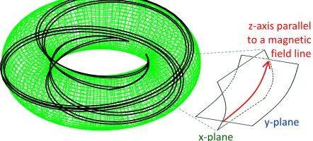
with concentric circular magnetic flux surfaces, whereqis the safety factor and the quantities with subscript 0 denotes the values at the center of the simulation domain. While plasma turbulence has short perpendicular wavelengths, its structure elongates in the direction parallel to the magnetic field. Therefore, a long and thin simulation domain along magnetic field lines is suitable for capturing the nature of plasma turbulence with reducing computational costs. An example of this flux-tube simulation domain is shown in Fig. 1, which is written by the projection of a box with short lengths inxandyand a long length inz. The flux-tube model is widely used to analyze turbulent transport in the local approximation limit, where the equilibrium quan-tities are given by local values.
By assuming statistically homogeneous turbulent fields, we impose periodic boundary conditions in xand
yand apply the Fourier decomposition as
φ(x, y,z)= kx ky
φkx,ky(z) exp
i(kxx+kyy)
. (5)
Additionally, there is the physical periodicity in the poloidal angleθas φ(r, θ, ζ) =φ(r, θ+2π, ζ). This leads the modified periodic boundary condition along the field-aligned coordinatez,
φkx,ky(z)= Θφkx+Δ,ky(z+2π), (6) where the connection phaseΘ =exp(i2πkyr0) and
connec-tion wave numberΔ = −2πs0ky with the poloidal wave
numberkyand the magnetic shears0[14].
The equations (1)-(3) are numerically solved in (kx,ky,z, v, μ) space except the nonlinearE×Badvection term. Since direct calculations of nonlinear convolutions in wave number space are computationally too expensive, theE×Badvection term is evaluated in the real space and transformed back to the wave number space by means of the 2D FFT and the 3/2 de-aliasing rule in (kx,ky).
3. Parallelization for Peta-Scale
Com-puting
To attain good performance on a distributed-memory system, domain decomposition by using a MPI library is necessary, as well as thread parallelization. The original GKV code decomposes 5D phase space in three directions (z, v, μ), which is not enough for multi-scale turbulence simulations. In order to achieve efficient computations on peta-scale supercomputers, we additionally decompose perpendicular wave-number spacek =(kx,ky) and imple-ment overlaps of computations and inter-node communi-cations.
3.1
Domain decomposition
At the beginning, we briefly explain the paralleliza-tion in (z, v, μ). The simulation domain is straightfor-wardly decomposed in 3D subdomains. Each subdomain has additional border cells to evaluate partial derivatives in (z, v, μ) by using finite difference methods. The dominant communications are only six point-to-point communica-tions between adjacent subdomains, which leads to excel-lent scaling. This 3D domain decomposition has already been implemented in the original GKV code. Extension to the 4D decomposition is done by performing the following wave-number-space decomposition on each subdomain in (z, v, μ).
Now, we consider the 2D FFT inkxandky, which are parallelized inkyandkx(x), respectively. Then, theE×B advection term is evaluated by using the 1D FFT in the following way:
• IF-X: 1D inverse FFT inkxwithky-decomposition.
• TR-XY: Data transpose fromky-decomposition to x-decomposition.
• IF-Y: 1D inverse FFT inkywithx-decomposition.
• RSC: Calculation of theE×Bterm in real space (x, y).
• FF-Y: 1D FFT inywithx-decomposition.
• TR-YX: Data transpose fromx-decomposition toky
-decomposition.
• FF-X: 1D FFT inxwithky-decomposition.
For convenience, the abbreviations will be used through-out this paper. The inter-node transpose communications are implemented by usingMPI_ALLTOALL, and the other terms are also parallelized in (ky,z, v, μ). We note that above wave-number space decomposition is better than another decomposition [i.e., (kx,ky) space is decomposed inkx and (x, y) space is decomposed in y], which intro-duces extra point-to-point communications inkx to apply the modified periodic boundary condition, Eq. (6). Since the distance of the mode connection is proportional toky,
the number of the extra communications increases as res-olutions or the number of parallelization in perpendicular wave-number space increase. Thus, the extra communica-tions may degrade scalability if we employ the latter de-composition.
We use a FFT library, FFTW3 [15], for computing FFTs and employ a parallel de-aliasing strategy similar to that shown in Ref. [7]. For applying the 3/2 de-aliasing rule, kx-direction is expanded before the nonlinear term calculation, andky-direction is expanded just after the first
data transpose. Similarly, truncation inkyis carried out
be-fore the second transpose, while truncation inkx is done after the nonlinear term calculation. Since expansion and truncation in ky are embedded in the parallel de-aliased
spectral calculations, the costs of expansion and truncation inkxonly appear explicitly in the cost analysis (see Fig. 3 in Sec. 4).
3.2
Overlaps of FFTs and transpose
Table 1 Overlap methods of FFTs and transpose. For simplicity, we use following abbreviations, IF-X (or -Y): Inverse FFT inx(ory), TR-XY (or -YX): Transpose communications fromky(orkx) -decomposition tokx(orky) -decomposition, RSC: Calculations of
theE×Badvection term in real space, and FF-X (or -Y): Forward FFT inx(ory). Asterisks representμ-loop and “(i)” denotes number ofμ-loop.
No overlap Partial overlaps Integrated overlaps
(μ-loop splitting and overlaps of each (μ-loop splitting and overlaps of all routines.) transpose and neighboring FFTs.)
* IF-X(i) IF-X(1) IF-X(1)
* TR-XY(i) TR-XY(1), IF-X(2) TR-XY(1), IF-X(2)
* IF-Y(i) * TR-XY(i), IF-X(i+1), IF-Y(i−1) TR-XY(2), IF-X(3), IF-Y(1)
* RSC(i) TR-XY(n), IF-Y(n−1) * TR-XY(i), IF-X(i+1), IF-Y(i−1), RSC(i−2)
* FF-Y(i) IF-Y(n) TR-XY(n), IF-Y(n−1), RSC(n−2), FF-Y(1)
* TR-YX(i) * RSC(i) TR-YX(1), FF-Y(2), IF-Y(n), RSC(n−1)
* FF-X(i) FF-Y(1) TR-YX(2), FF-Y(3), FF-X(1), RSC(n)
TR-YX(1), FF-Y(2) * TR-YX(i), FF-Y(i+1), FF-X(i−1) * TR-YX(i), FF-Y(i+1), FF-X(i−1) TR-YX(n), FF-X(n−1)
TR-YX(n), FF-X(n−1) FF-X(n)
FF-X(n)
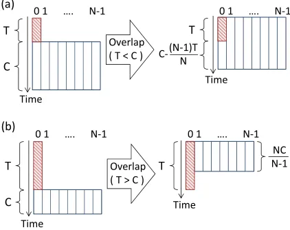
Fig. 2 Schematic pictures of the overlap method with MPI/OpenMP hybrid parallelization with N threads in the cases that (a) the communication costT is smaller than the computational costC, and (b)T is larger than C. The zeroth thread works as a communication thread, and the others work as computation threads. Shaded and unshaded boxes represent communication and computation tasks, respectively.
and computations, which are independent of the commu-nication data, on the other threads are carried out at the same time. To reduce load imbalance, the computations are parallelized by means ofDYNAMICloop decompositions, where the chunk size is set to be 1 to decrease the granu-larity. The master thread can also carry out computations after communications end, if the communication costs are smaller than the computational costs. On the other hand, if communication costs are larger than computational ones, computation threads finish their works and wait until the
communications end. Thus, the total cost S with the over-lap of computations and communications is,
S = ⎧⎪⎪ ⎪⎪⎨ ⎪⎪⎪⎪⎩ C+
T N
T ≤ NC
N−1
T
T > NC N−1
, (7)
where N, T andC are the number of OpenMP threads, communication and computational costs without overlaps, respectively. We note that this is an ideal estimation, be-cause computation tasks may not be uniformly parallelized by both ofN andN−1 threads, which leads load imbal-ance and increases computational costs. While both cases in Fig. 2 show reductions of computational costs compared to the cost in the case without overlap,C+T, the case of T <Cis preferable from the view point of efficient use of computational resources. Therefore, it is important to find as many computing sections which are independent of the communication data as possible to improve scalability.
Fig. 3 Histogram of the elapsed time in the case without over-laps (where the number of the wave-number-space par-allelization is 32). The items named “E×B”, “Linear”, and “Others” correspond to the computational costs of the
E×Badvection term, linear terms and communications in (z, v, μ), and the rest including a field solver. Abbre-viations are same as Table 1 except IN: Expansion inkx
before data input to a FFT library, and OUT: Truncation inkxof the output data from a FFT library.
parts of IF-X and FF-X, and the whole computation be-tween the two transpose communications. Since the latter increases overlapped computations, the integrated overlaps are more promising to improve scalability than the partial overlaps.
4. Performance Analysis
We analyze effects of the presented overlap meth-ods on the strong scaling of the calculation of the E× B advection term. Computations shown in this section were carried out on the FX10 supercomputer (SPARC64 IXfx 1.848 GHz, 14.78 GFlops/core, Memory bandwidth 5.3 GB/s/core, 16 cores/node, 6D Mesh/Torus intercon-nect, Interconnect bandwidth 5 GB/s×4, 4800 nodes) in the University of Tokyo. In the following results, we em-ploy 1024×1024×16×16×16 grid points, which are scaled down from those required for multi-scale turbulence simulations, and decompose into 8(16,32,64)×2×2×2 subdomains. Each subdomain has a MPI process and eight OpenMP threads.
4.1
Analysis of computational costs
Before comparing the overlap methods, it is useful to check the computational costs of the target calculation without overlaps. Figure 3 shows the histogram of the computational cost of the GKV code employing the wave-number-space decomposition without overlaps of compu-tations and communications. The calculation of theE×B advection term accounts for 66% of the total computational cost, and the costs of transpose communications and FFTs are dominant. In Fig. 4, elapsed time of theE×Badvection
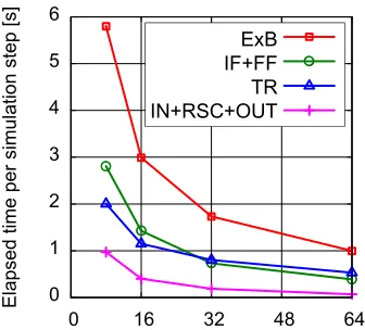
Fig. 4 Elapsed time of theE×Badvection term calculation in the case without overlaps as a function of the number of wave-number-space parallelization. Elapsed time of to-talE×Bterm calculation, Fourier transform, transpose communications and the others are plotted with square, circular, triangle and cross dots, respectively.
term calculation is plotted as a function of the number of the wave-number-space parallelization. It is clearly shown that the cost of transpose communications decreases more slowly than that of computations. The cost of communica-tions tends to be dominant as the number of wave-number space parallelization increases, and degrades scalability. In the case shown here, the cost of communications exceeds that of FFTs when the number of wave-number space par-allelization is larger than 32, where the partial overlaps are not enough to mask communications.
Using Eq. (7), one can estimate the elapsed time in the case with the integrated overlaps from the data without overlaps. Since IF-X(0) and FF-X(n) are not overlapped, the estimation is given by
Sint=
⎧⎪⎪⎪ ⎪⎨ ⎪⎪⎪⎪⎩
CIF−X+CFF−X
n +Ceff+
T N
T ≤ NCeff N−1
CIF−X+CFF−X
n +T
T > NCeff N−1
,
(8) whereCeff=(n−1)(CIF−X+CFF−X)/n+CIF−Y+CRSC+CFF−Y
represents the effectively overlapped computational cost, and to simplify the problem, we only consider two cases: all communications are completely masked or not masked. When the data input and output for a FFT library are also included in the overlaps, the estimation becomes
Sint=max
C+ T
N,
CIN+CIF−X+CFF−X+COUT
n +T
.
Fig. 5 Elapsed time of theE×Badvection term calculation as a function of the number of wave-number-space paral-lelization. Square, circular and triangle dots correspond to the cases without overlaps, with the partial overlaps, and with the integrated overlaps, respectively. The esti-mation of the elapsed time in the case with the integrated overlaps, Eq. (9), is plotted as a dashed line.
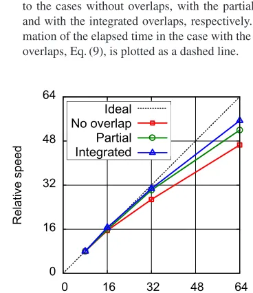
Fig. 6 Strong scaling of theE×Badvection term calculation. The relative speeds (which are proportional to inverse of the elapsed time) in the cases without overlaps, with the partial overlaps, and with the integrated overlaps are plot-ted with square, circular, triangle dots, respectively. The dotted line represents the ideal speed up for reference.
4.2
E
ff
ects of the overlap methods
Elapsed time of the E×B advection term calcula-tion in the cases without overlaps, with partial overlaps, and with integrated overlaps is plotted as a function of the number of wave-number-space parallelization in Fig. 5. The estimation of the elapsed time in the case with the in-tegrated overlaps shows good agreements with the mea-sured values, which assures that the integrated overlaps are successfully implemented with the smallest load im-balance. For example, the detailed time measurement for the case without overlaps records the computational cost
Table 2 Comparison of the performance of the E×B advec-tion term calculaadvec-tion between the cases without over-laps, with the partial overover-laps, and with the integrated overlaps (where the number of the wave-number-space parallelization is 32).
TFlops Peak ratio
No overlap 1.21 4.01%
Partial overlaps 1.86 6.17% Integrated overlaps 1.97 6.54%
C = 1.827 s, the communication costT = 1.149 s and Ceff =(n−1)(CIN+CIF−X+CFF−X+COUT)/n+CIF−Y+CRSC+
CFF−Y = 1.738 s, when the number of the
wave-number-space parallelization is 16, the number of OpenMP threads N=8 and the number of the pipelined loopsn=8. Since T <NCeff/(N−1), it is expected that the integrated
over-laps efficiently mask the communication cost. The elapsed time for the integrated overlaps is 1.968 s, which is the same as the estimated value (Sint = C+T/N =1.971 s)
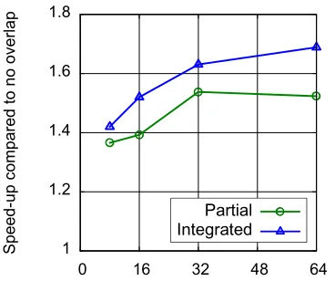
Fig. 7 Speed-up compared to the case without overlaps as a function of the number of wave-number-space paral-lelization. The circular and triangle dots correspond to the cases with partial and integrated overlaps, respec-tively.
Fig. 8 Strong scaling test of the GKV code on the K computer [where 1024×1024×64×64×32 grid is decomposed into 8(16,32,64)×8×8×4 subdomains and each subdomain employs 8 threads]. Square and triangle dots correspond to the cases without overlaps and with the integrated over-laps on theE×Bterm calculation, respectively.
5. Strong Scaling beyond 100 k Cores
We examine the impact of the developed overlap method on the total performance of the GKV code. The following computations are carried out on the K computer (SPARC64 VIIIfx 2 GHz, 16 GFlops/core, Memory band-width 8 GB/s/core, 8 cores/node, 6D Mesh/Torus intercon-nect, Interconnect bandwidth 5 GB/s×4, 88128 nodes), employing the resolution required for the multi-scale tur-bulence simulations.
Figure 8 shows the strong scaling of the GKV code on the K computer. The domain decomposition in per-pendicular wave number space allows us to employ more than 100 k cores, and the integrated overlaps significantly
improve the strong scaling. In addition, the process map-ping on a 3D torus network is optimized so that the trans-pose communications are performed among the neighbor-ing nodes located in a 3D box shape, which maximize a bi-section bandwidth available on the torus network, and reduces costs ofMPI_ALLTOALL. Thanks to the above op-timization techniques, the GKV code achieves almost lin-ear speed-up beyond 100 k cores. The parallel efficiency estimated from the Amdahl’s law is 99.9998%, which is improved by an order of magnitude compared with the pre-vious results (∼99.998% evaluated from Fig. 2 shown in Ref. [16]). The effect of the overlaps becomes more signif-icant as the number of cores increases. The case with the integrated overlaps achieves 168 TFlops (8.03% of the the-oretical peak performance) at 131,072 cores, which is 29% higher performance than that in the case without overlaps. To further speed up the GKV code, additional tuning for serial and parallel algorithms will be performed in near fu-ture.
6. Conclusion
We have presented a massively-parallelized gyroki-netic Vlasov simulation code GKV, which is developed to study turbulent transport in magnetically-confined plas-mas. To address multi-scale turbulence simulations, the parallelization of the GKV code has been extended to make it run efficiently on peta-scale supercomputers in two steps. First, three-dimensional domain decomposition has been extended to four-dimensional one to increase the num-ber of available processes. This extension introduces ad-ditional inter-node transpose communications to calculate the nonlinearE×Badvection term, which degrades scal-ability. Second, overlaps of computations and communi-cations have been implemented to improve scalability by means of MPI/OpenMP hybrid parallelization. The inte-grated overlaps of whole calculations of theE×B advec-tion term show better strong scaling than that in the case with partial overlaps of each transpose and neighbor FFTs, and achieves speed-up by 63% of that in the case with-out overlaps. The completed two extensions significantly improve scalability of theE×Badvection term and make substantial speed-up. The strong scaling test on the K com-puter demonstrates that the extended GKV code is easily scaled up beyond 100 k cores and able to realize efficient computations of multi-scale turbulence simulations.
Acknowledgments
This work is performed with supports of the HPCI Strategic Program for Innovative Research and the JAEA-NIFS Collaboration Program. A part of the results is ob-tained by early access to the K computer at the RIKEN Advanced Institute for Computational Science. One of the authors (S.M.) would like to thank H. Inoue and S. Tsut-sumi for their supports to implement the parallel FFT al-gorithm.
[1] X. Garbet, Y. Idomura, L. Villard and T.-H. Watanabe, Nucl. Fusion50, 043002 (2010).
[2] T.-H. Watanabe and H. Sugama, Nucl. Fusion 46, 24 (2006).
[3] D.G. Fox and S.A. Orszag, J. Comput. Phys. 11, 612 (1973).
[4] J.W. Cooley and J.W. Tukey, Math. Comput. 19, 297 (1965).
[5] C. Calvin, Parallel Comput.22, 1255 (1996).
[6] Z. Yin, L. Yuan and T. Tang, J. Comput. Phys.210, 325 (2005).
[7] M. Iovieno, C. Cavazzoni and D. Tordella, Comput. Phys.
Commun.141, 365 (2001).
[8] P. Wapperom, A.N. Beris and M.A. Straka, Parallel Com-put.32, 1 (2006).
[9] A. Danalis, K.Y. Kim, L. Pollock and M. Swany, Proc. IEEE/ACM Int. Conf. High Perform. Comput. (SC2005), Seattle, USA, pp. 58 (2005).
[10] P.D. Mininni, D. Rosenberg, R. Reddy and A. Pouquet, Par-allel Comput.37, 316 (2011).
[11] T. Adachi, N. Shida, K. Miura, S. Sumimoto, A. Uno, M. Kurokawa, F. Shoji and M. Yokokawa, Comput. Sci. Res. Dev.28, 147 (2013).
[12] Y. Idomura, M. Nakata, S. Yamada, M. Machida, T. Ima-mura, T.-H. Watanabe, M. Nunami, H. Inoue, S. Tsutsumi, I. Miyoshi and N. Shida, Int. J. High Perform. Comput. Appl., DOI: 10.1177/1094342013490973 (2013).
[13] S. Maeyama, A. Ishizawa, T.-H. Watanabe, N. Nakajima, S. Tsuji-Iio and H. Tsutsui, Comput. Phys. Commun., DOI: 10.1016/j.cpc.2013.06.014 (2013).
[14] M.A. Beer, S.C. Cowley and G.W. Hammett, Phys. Plasmas 2, 2687 (1995).
[15] M. Frigo and S.G. Johnson, Proc. IEEE93, 216 (2005). [16] T.-H. Watanabe, Y. Todo and W. Horton, Plasma Fusion