Comparison Study of Sorting Techniques in Static Data Structure

(1)

Comparison Study of Sorting Techniques in Static Data

Structure

Anwar Naser Frak

1

, Mohd Zainuri Saringat

1*

, Yuli Adam Prasetyo

2

, Aida

Mustapha

1

, Hannani Aman

1

, Noraini Ibrahim

1

Faculty of Computer Science and Information Technology, Universiti Tun Hussein Onn Malaysia, 86400, Johor, Malaysia

2

School of Computing, Telkom University, 40257 Bandung, West Java, Indonesia Received 28 June 2018; accepted 5August 2018, available online 24 August 2018

1. Introduction

Data structure is important to systematically organize large data in a computer system. A correct selection of data structures drives towards efficient implementation, making it suitable for various applications [1]. In addition, data structure is considered as a key and essential factor when designing effective and efficient algorithms [2, 3]. In the realm of software design, there are several studies that have attested the importance of data structures. Data structures are generally based on the ability of a computer to fetch and store data at any place in its memory, specified by a pointer with a bit stringer presenting a memory address. Thus, data structures concern on computation of the data item addresses via arithmetic operations. To date, there are various studies that demonstrate the importance of data structures in software design [4, 5].

Given a specific data structure, data management needs to involve a certain sorting process [6]. Sorting refers to ordering data in an increasing or decreasing fashion according to some linear relationship among the data items in a particular data structure. Sorting techniques have attracted a great deal of research for efficiency, practicality, performance, complexity and types of data structures [7, 8]. Rigorous efforts have been taken to improve sorting techniques like merge sort, bubble sort, insertion sort, quick sort, selection sort, and each of them has a different mechanism to reorder elements which increase the performance and

efficiency of the practical applications as well as reducing the time complexity for each one.

Nonetheless, while many research focused on improving the sorting algorithms, very little effort focuses on the types of data structure used on the sorting algorithms. Finding the most efficient sorting technique involves examining and testing these techniques to finish the main task as soon as possible and identifying the most suitable structure for sorting in shortest time. It is worth noting that when various sorting algorithms are being compared, there are a few parameters that must be taken into consideration, such as complexity, and execution time [9, 10]. The complexity is determined by the time taken for executing the algorithm [11]. In general, the time complexity of an algorithm is written in the form of Big O(n) notation, where O represents the complexity of the algorithm and the value n represents the number of elementary operations performed by the algorithm. Thus, the aim is to evaluate the efficiency of different sorting algorithms and study the factors that affect the practical performance of each algorithm in terms of its overall run time.

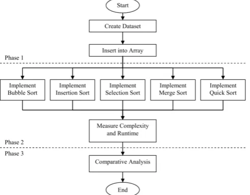
This paper investigates the efficiency of five sorting techniques; selection, insertion, bubble, quick and merge sort, as well as their behaviours on small and large data set. To accomplish these tasks, this research proposed a methodology that comprises of three phases, which are (1) implementation of sorting technique, (2) Abstract: To manage and organize large data is imperative in order to formulate the data analysis and data processing efficiency. Therefore, this paper investigates the set of sorting techniques to observe which technique to provide better efficiency. Five types of sorting techniques of static data structure, Bubble, Insertion, Selection with O(n2) complexity and Merge, Quick with O(n log n) complexity have been used and tested on four groups between (100–30000) of dataset. To validate the performance of sorting techniques, three performance metrics which are time complexity, execution time and size of dataset were used. All experimental setups were accomplished using simple linear regression. The experimental results illustrate that Quick sort is more efficiency than other sorting and Selection sort is more efficient than Bubble and Insertion in large data size using array. In addition, Bubble, Insertion and Selection have good performance for small data size using array thus, sorting technique with behaviour O(n log n) is more efficient than sorting technique with behaviour O(n2) using array

.

(2)

calculation of their complexity, and finally (3) comparative analysis. Each phase contains different steps and delivers useful results to be used in the next phase. Finally, performance of all five sorting techniques were evaluated by three performance measures which are time complexity, execution or run time and size of dataset used.

The remainder of this paper proceeds as follows. Section 2 presents the related work pertaining to sorting algorithms. Section 3 presents the research methodology, Section 4 discusses the comparative analysis and finally Section 5 concludes with some indication for future work.

2. Related Work

A considerable amount of literature has been published on sorting techniques. While looking into large and growing body of literature, it is appeared that sorting techniques have been proven to be successful for data structures. Thus, the data structures have an impact on the efficiency of these sorting techniques. [5] discussed and reviewed the performance of sorting techniques where comparisons of the algorithms were based on the time of implementation. It was found that for small data, the six techniques perform well, but for large input data, only quick sort and grouping comparison sort (GCS) are considered fast. [10] examined several sorting algorithms and discussed the performance analysis of these sorting algorithms based on their complexity while testing them with list data structure. It was found that the merge sort and quick sort have high complexity but faster in large lists.

In the work of [1], four techniques which are insertion sort, quick sort, heap sort and bubble sort were compared. Although all these techniques are of O(n2) complexity, it was found that they produced different results in execution time with quick sorting technique being the most efficient in terms of execution time. [14] proposed a new sorting algorithm named “index sort” and evaluate its performance by making comparison with other four sorting techniques; insertion sort, bubble sort, selection sort and merge sort, based on their running time. The research found that the proposed index sort is faster than the other sorting algorithms.

In general, bubble sort is a simple and the slowest sorting algorithm which works by comparing each element in the list with progress elements and swapping them if they are in undesirable order. The algorithm continues this operation until it makes a pass right through the list without swapping any elements, which shows that the list is sorted. This process takes a lot of time and especially slow when the algorithm works with a large data size. Therefore, it is considered to be the most inefficient sorting algorithm with large dataset [5]. Insertion sort is a simple and efficient sorting algorithm, beneficial for small size of data. It works by inserting each element into its suitable position in the final sorted list. For each insertion, it takes one element and finds the suitable position in the sorted list by comparing with contiguous elements and inserts it in that position [6].

Quick sort uses divide and conquer method for solving problems. It works by partitioning an array into two parts, then sorting the parts independently. It finds the elements called pivot which divides the array into halves in such a way that elements in the left half are smaller than the pivot, and elements in the right half are greater than pivot [5]. Selection sort works by selecting the highest element needed to compare all n elements in the list at first iteration and swapping them if required. Likewise, to select the next highest element it needs to compare n elements in the list and so on. Hence it requires O(n2) comparisons and n-1 swaps to sort the list of n elements. Since it has the worst case running time of O(n2) [11].

Finally, merge sort works by dividing and conquering the Merge sort, dividing the array in two halves at each stage, which gives it lg(n) component and the other N component derived from its comparisons that are made at each stage. Therefore combining it becomes nearly O(n log n) which in the worst case, merge sort requires O(n log n) time to sort an array with n elements [5].

3. Methodology

The objective of this paper is to analyse the performance of five sorting algorithms in a static data structure, which is array. An array is the arrangement of data in the form of rows and columns that is used to represent different elements through a single name but different indicators, thus, it can be accessed by any element through the index [4]. Arrays are useful in supplying an orderly structure which allows users to store large amounts of data efficiently. For example, the content of an array may be changed during runtime whereas the internal structure and the number of the elements are fixed and stable. An array could be called fixed array because they are not changed structurally after they are created. This means that the user cannot add or delete to its memory locations (making the array having less or more cells), but can modify the data it contains because it is not change structurally. The research framework in three phases is shown in Fig. 1.

(3)

The first phase is implementation of the sorting algorithms, which are bubble sort, insertion sort, selection sort with O(n2) complexity, as well as merge sort and quick sort with O(log n) complexity. The second phase is calculating the complexity of these five sorting algorithms. According to [12], the time complexity of an algorithm quantifies the amount of time taken by an algorithm to run as a function with the length of a string representing the input. Execution time is the time taken to hold processes during the running of a program. The speed of the implementation of any program depends on the complexity of a technique or algorithm. If the complexity is low, then the implementation is faster, whereas when the complexity is high then the implementation is slow [13]. The time complexity of an algorithm is commonly expressed using Big(O) notation, which excludes coefficients and lower order terms. The time complexity is commonly estimated by counting the number of elementary operations performed by the algorithm, where an elementary operation takes a fixed amount of time to perform.

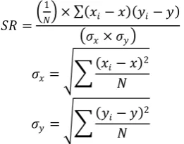
The third phase is comparing and analysing these sorting algorithms with performance measurement execution time per second, and size of the dataset, based on simple linear regression. Regression analysis is a statistical function used to find the estimated value between variable groups, which includes many of the techniques that are used in special preparation analysed to determine the relationship between the dependent and independent variable.

In this experiment, a least square estimator of a linear regression model with a single explanatory variable was used. In this model, there exists a simple straight line which passes through a series of dots that make total residuum any distance between the real point and the estimated point. Regression analysis used to predict or find a relationship between the independent variable and dependent variable moreover, its impact on the dependent variable. Thus regression analysis finds a causal relationship between the variables [8]. The linear regression equation is shown in Equation 1.

𝑌𝑌 = 𝑎𝑎 + 𝑏𝑏 × 𝑋𝑋 (1)

where Y is the dependent variable, X is the independent variable, a is the constant (or intercept), and b is the slope of the regression line. The equation of squares regression is shown in Equation 2.

𝑆𝑆𝑆𝑆 =� 1

𝑁𝑁� × ∑(𝑥𝑥𝑖𝑖− 𝑥𝑥)(𝑦𝑦𝑖𝑖− 𝑦𝑦) �𝜎𝜎𝑥𝑥× 𝜎𝜎𝑦𝑦�

(2)

𝜎𝜎𝑥𝑥= ��(𝑥𝑥𝑖𝑖− 𝑥𝑥) 2 𝑁𝑁

𝜎𝜎𝑦𝑦 = ��(𝑦𝑦𝑖𝑖− 𝑦𝑦) 2 𝑁𝑁

where N is the number of observations used to fit the model, Xi is the x value of observation i, Yi is the yvalue

of observation i, Y is the mean y value, 𝜎𝜎_𝑥𝑥is the standard deviation of x, and 𝜎𝜎_𝑦𝑦 is the standard deviation of y. Following [9], a ratio is a relationship between two numbers indicating how many times the first number contains the second number. The equation of ratio is shown in Equation 3.

𝑠𝑠𝑠𝑠𝑠𝑠𝑠𝑠𝑠𝑠 ≈_{𝑠𝑠𝑠𝑠𝑒𝑒𝑖𝑖𝑒𝑒𝑎𝑎𝑒𝑒𝑠𝑠𝑠𝑠 𝑣𝑣𝑎𝑎𝑣𝑣𝑣𝑣𝑠𝑠 𝑓𝑓𝑓𝑓𝑓𝑓 𝑎𝑎𝑣𝑣𝑎𝑎𝑓𝑓𝑓𝑓𝑖𝑖𝑒𝑒ℎ𝑒𝑒 2}estimated value for algorithm 1 (3)

4. Experiments and Results

During the implementation phase, all the sorting algorithms were implemented to sort four groups of datasets between 100 to 30,000 lines. The hardware requirements included C++ programming language, an Intel (R) Core (TM) 2 Duo CPU E8400 operating system at 3.00 GHz (2 CPUs), along with installed memory (RAM) of 2,038 MB. In this study, static data structure was used. The instance of the array structure is fixed and remain static throughout the program run time. The content of the array used may be changed during the execution, but the internal structure and the number of elements in the structure remain unchanged. Table 1 to Table 4 show the experimental result of execution time for four groups.

Table 1: Results of Execution Time for Group 1 n= (100 to 1000)

n

O(n2) Group O(n log n) Group Bubbl

e

Insertio n

Selectio n

Merge Quick

100 0 0 0 0 0

200 0 0 0 0 0

300 0.001 0 0.001 0 0

400 0.001 0 0.001 0 0

500 0.001 0.001 0.001 0 0

600 0.001 0.001 0.001 0 0

700 0.002 0.001 0.001 0 0

800 0.002 0.001 0.001 0 0

900 0.002 0.001 0.002 0 0

1000 0.003 0.002 0.002 0 0

Est.

Value 0.001 35

0.0007 0.00103 0 0

Table 2: Results of Execution Time for Group 2 n= (2000 to 10,000)

n

O(n2) Group O(n log n) Group Bubble Insert

ion

Selecti on

Merge Quick

2000 0.015 0.006 0.008 0 0

3000 0.028 0.014 0.017 0.001 0 4000 0.053 0.026 0.031 0.001 0

5000 0.087 0.04 0.047 0.001 0

6000 0.131 0.058 0.069 0.001 0.001 7000 0.205 0.079 0.100 0.001 0.001 8000 0.257 0.105 0.131 0.001 0.001 9000 0.346 0.136 0.166 0.002 0.001 10000 0.454 0.177 0.217 0.002 0.001 Est.

(4)

5 1

Table 3: Results of Execution Time for Group 3 n= (11000 to 20000)

n

O(n2) Group O(n log n) Group Bubbl

e

Insertio n

Select ion

Merge Quick 11000 0.527 0.227 0.252 0.002 0.001 12000 0.635 0.241 0.295 0.003 0.002 13000 0.752 0.278 0.352 0.003 0.002 14000 0.868 0.343 0.41 0.003 0.002 15000 1.043 0.386 0.483 0.003 0.003 16000 1.178 0.454 0.541 0.003 0.003 17000 1.351 0.557 0.604 0.004 0.003 18000 1.501 0.564 0.712 0.004 0.003 19000 1.659 0.633 0.757 0.004 0.003 20000 1.862 0.697 0.845 0.005 0.003 Est.

Value 0.5757 0.5118 0.385 0.00515 0.0037

Table 4: Results of Execution Time for Group 4 n= (21000 to 30000

n

O(n2) Group O(n log n) Group

Bubble Inserti

on

Selectio n

Merge Quick

21000 2.105 0.786 0.944 0.005 0.003

22000 2.244 0.859 1.014 0.005 0.004

23000 2.428 0.962 1.122 0.005 0.004

24000 2.668 1.012 1.22 0.006 0.004

25000 2.937 1.096 1.297 0.006 0.004

26000 3.203 1.197 1.473 0.006 0.005

27000 3.502 1.297 1.538 0.007 0.005

28000 3.958 1.384 1.683 0.007 0.005

29000 4.089 1.506 1.855 0.007 0.005

30000 4.22 1.703 2.027 0.007 0.005

Est.

Value 4.2376 1.281 0.943 0.00855 0.006

5. Comparative Analysis

Five sorting techniques were compared in a series of four-group experiments using dataset of different sizes. The dataset was implemented as array. To appraise the obtained results, linear regression was used. The linear regression method is used to generate estimators and other statistics in regression analysis. Besides, the method of linear regression is a standard approach in regression analysis to approximate solution. The estimated value and ratio value for each measurement is considered as comparison criteria in this study.

A minimum estimated value (constant factors) indicates a fitting linear and the best fit in the linear regression. A minimum percentage of the ratio indicates that the execution time is not affected when size of data is increased [9]. The comparative analysis is based on theestimated value of execution time per second for

each sorting technique according to each group as shown in Table 5.

Table 5: Experimental Results for Four Groups Based on Estimated Value

Sorting Algorith m

Estimated Value Avg. Est. Value Grou

p 1

Group 2

Grou p 3

Group 4 Bubble

Sort

0.001 0.127 0.576 4.238 1.235 Insertion

Sort

0.001 0.0565 0.512 1.281 0.463 Selection

Sort

0.001 0.099 0.385 0.943 0.357 Merge

Sort

0.000 0.001 0.005 0.009 0.004 Quick

Sort

0.000 0.001 0.004 0.006 0.003

Based on the experimental results, the analysis include (1) comparison of estimated value for each sorting algorithm in each group based on Equation [1], (2) comparison of average estimation value for each sorting algorithm, (3) comparison of average ratio between sorting algorithms within the same group as based on Equation [2], and finally (4) comparison of average ratio speed for every sorting algorithms between the group based on Equation [2].

A. Estimated Value for Each Sorting Algorithm

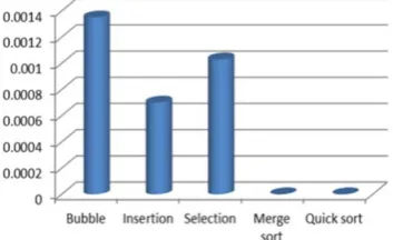
Comparison of the compared estimated value of Group 1 to Group 4 datasets (100-30000) for five sorting algorithms are shown in Fig. 2 to Fig. 5

.

Fig. 2 Estimated value for Group 1

(5)

B. Average Estimation Value for All Sorting Algorithms

The comparisons on the average estimated value for all groups data set of five sorting techniques are shown in Fig. 6. It is evident that there is a difference in efficiency between sorting techniques in terms of measurement of the data size and sorting time per second using array. The merge and quick sort have a minimum average for estimation value across all groups data set. Thus, it can be concluded that merge and quick sort are more efficient compared to bubble, insertion and selection sort. However, the selection sort is more efficient than bubble and insertion sort.

Fig. 6 Comparison of average estimated value of five sorting algorithms

C. Average Ration between Two Sorting Algorithms

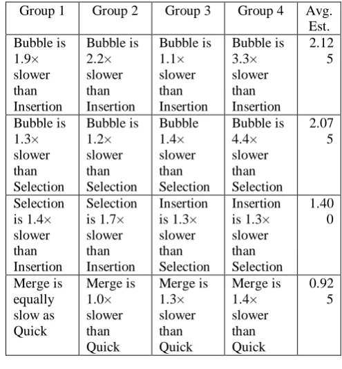
To determine the ratio of the variation between the speeds of the five sorting techniques, comparisons have been made by calculating the average of ratio of a sorting technique and compare it with other sorting technique in the same group. based on Equation 2. The results are shown in Table 6.

Table 6: Comparison of Ration of Variation Between Sorting Speed

Group 1 Group 2 Group 3 Group 4 Avg. Est. Bubble is 1.9× slower than Insertion Bubble is 2.2× slower than Insertion Bubble is 1.1× slower than Insertion Bubble is 3.3× slower than Insertion 2.12 5 Bubble is 1.3× slower than Selection Bubble is 1.2× slower than Selection Bubble 1.4× slower than Selection Bubble is 4.4× slower than Selection 2.07 5 Selection is 1.4× slower than Insertion Selection is 1.7× slower than Insertion Insertion is 1.3× slower than Selection Insertion is 1.3× slower than Selection 1.40 0 Merge is equally slow as Quick Merge is 1.0× slower than Quick Merge is 1.3× slower than Quick Merge is 1.4× slower than Quick 0.92 5

Fig. 7 shows the comparison of the variation between the ﬁve sorting techniques.

Fig. 7 Comparison of average ration between five sorting algorithms

Fig. 7 implies that there is a variation between the ratios of the ﬁve techniques in terms of measurement ratio. The merge sort and quick sort have a minimum average of ratio for variation in speed among ﬁve sorting techniques. This indicates that merge sort and

quick sort are most e ﬃcient in ter

using array. On the other hands, the bubble sort, insertion sort and selection sort have the maximum average ratio. This indicates that bubble sort, insertion

sort and selection sort are less e ﬃcient in ter sor

ting data using array.

D. Average Speed Ratio for Each Algorithm

Finally, comparison has been made among ﬁve sorting techniques based on the calculated average sorting speed ratio as stated in Equation 2. Table 7 shows the speed ratio between the techniques for

di ﬀerent data sizes.

(6)

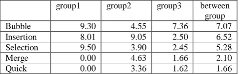
group1 group2 group3 between group

Bubble 9.30 4.55 7.36 7.07

Insertion 8.01 9.05 2.50 6.52

Selection 9.50 3.90 2.45 5.28

Merge 0.00 4.63 1.66 2.10

Quick 0.00 3.36 1.62 1.66

Based on Table 7, the comparison of average sorting speed ratio between groups has been made for ﬁve techniques as shown in Fig. 8. It demonstrates that there is a difference in percentage between sorting techniques in terms of measuring the average ratio sorting speed between the groups.

Fig. 8 Comparison of the average speed ratio between sorting algorithms

6. Conclusions

Based on the comparative analysis, quick sort has the smallest average ratio sorting speed that indicates that it is highly efficient when working with different data sizes implemented as arrays. Whereas, bubble sort, insertion sort and selection sort have maximum average ratio sorting speed between the groups which indicates that they are less efficient in terms of execution time.

On the whole, the comparative analysis signify that the variation was clear between groups of data and sorting techniques at different sizes of data set as well as sorting time per second. Merge sort and quick sort are more efficient in terms of minimum average estimation value and minimum average ratio sorting speed as compared to the remainder of the sorting techniques. On the contrary, bubble sort, insertion sort and selection sort have maximum average estimation value and maximum average ratio speed which means that they have poor efficiency when working with large datasets. It can be concluded that sorting techniques that have complexity of O(n log n) is more efficient than sorting techniques of complexity O(n2).

Acknowledgement

This project is sponsored by Universiti Tun Hussein Onn Malaysia.

References

[1] N. Chhajed, I. Uddin and S. S. Bhatia, “A comparison based analysis of four different types of sorting algorithms in data structures with their performances”, International Journal of Advance Research in Computer Science and Software Engineering, 3(2): 373-381, 2013.‏

[2] V. Okun, A. Delaitre and P. E. Black, “Report on the third static analysis tool exposition”, SATE, 500, 283, 2011.

[3] P. E. Black, “Dictionary of algorithms and data structures”, US National Institute of Standards and Technology, 2009.

[4] B. Andres, U. Koethe, T. Kroeger and F . A. Hamprecht, “Runtime-flexible multi -dimensional arrays and views for C ++ 98 and C++”, 0x. arXiv preprint arXiv:1008.2909, 2010.‏

[5] K. S. Kharabsheh, I. M. Turani, A. M. I. Al-Turani and N. I. Zanoon, “Review on Sorting Algorithms A Comparative Study”, International Journal of Computer Science and Security, 7(3):120, 2013.

[6] Y. Liu and Y. Yang, “Quick-merge sort algorithm based on Multi-core linux”, in Proceedings of the International Conference in Mechatronic Sciences, Electric Engineering and Computer, 1578-1583, 2013.

[7] A. A. Voevoda and D. O. Romannikov, “A Binary Array Asynchronous Sorting Algorithm with Using Petri Nets”, Journal of Physics: Conference Series, 803(1):012178, 2017.

[8] A. J. Umbarkar, U. T. Balande and P. D. Seth, “Performance evaluation of firefly algorithm with variation in sorting for non-linear benchmark problems”, in Proceedings of the AIP Conference Proceedings, 1836(1):020032, 2017.

[9] D. Rajagopal and K. Thilakavalli, “Different Sorting Algorithm’s Comparison based Upon the Time Complexity”, International Journal of u-and e-Service, Science and Technology, 9(8):287—296, 2016.

[10] N. Chowdhury, “A Java Based Tool to Monitor Execution Time of Different Sorting Algorithms”, Doctoral dissertation, East West University (2016). [11] M. Goodrich, R. Tamassia and D . Mount, “Data

structures and algorithms in C ++”, John Wiley & Sons, 2007.‏

[12] W. Waegeman, B. D. Baets and L. Boullart, “ROC analysis in ordinal regression learning”, Pattern Recognition Letters Pattern Recognition Letters, 29(1):1-9, 2008.

[13] C. K. Shene, “A Comparative Study of Linkedlist Sorting Algorithms”, Department of Computer Science, Michigan Technological University, Houghton, 1996.

(7)

[15] S. Abdel-Hafeez and A. Gordon-Ross, “An Efficient O(N) Comparison-Free Sorting Algorithm”, in Proceedings of the IEEE Transactions on Very Large Scale Integration (VLSI) Systems, 25(6): 1930-1942, 2017.

[16] A. R. Estakhr, “Physics of string of information at high speeds, time complexity and time dilation”, Bulletin of the American Physical Society , 58, 2013.‏

[17] P. P. Puschner and C. Koza, “Calculating the maximum execution time of realtime programs”, Real-Time Systems, 1(2):159-176, 1989.