EVALUATION OF NONLINEARITY
EFFECTS ON PERFORMANCE OF
DVB-H TRANSMISSION LINK
MD. SARWAR MORSHED
Computer Science and Information Technology Department, Islamic University of Technology, Board Bazar, Gazipur-1704, Bangladesh
[email protected] http://www.iutoic-dhaka.edu
HASAN MAHMUD
Computer Science and Information Technology Department, Islamic University of Technology, Board Bazar, Gazipur-1704, Bangladesh
[email protected] http://www.iutoic-dhaka.edu S. M. DIDAR-AL-ALAM
Computer Science and Information Technology Department, Islamic University of Technology, Board Bazar, Gazipur-1704, Bangladesh
[email protected] http://www.iutoic-dhaka.edu Abstract:
Handheld devices of all kind have gained remarkable popularity in recent years. Choosing receiving end components for these handheld devices are critical. For example, if poorly suited and inexpensive amplifiers are chosen, then they tend to deteriorate signals. On the other hand, cheaper components are feasible for consumer product. This paper evaluates nonlinearity effects on transmission link serving Digital Video Broadcasting for Handhelds (DVB-H) based on the results of software simulator. The system is tested in various receiving scenarios with presence of noise and received signal power varying from sensitivity level up to saturated nonlinear region. Neighboring DVB-H channel and close-by GSM-uplink are considered as distortion sources. The simulation results also analyze the behavior of the system in the presence of interfering signals with various power levels.
Keywords: DVB-H; Nonlinearity; DVB-T.
1. Introduction
DVB-H is the standard introduced to meet the requirements of digital TV broadcasting for handheld devices. It is the extended version of Digital Video Broadcasting – Terrestrial (DVB-T) and thus offers even some backwards compatibility. After the success that DVB-T had around the world, this new DVB-H standard appears to be promising as it has already been proven effective in many commercial and trial deployments. Because DVB-T is already widely spread, implementation of the DVB-H transmission system on top of that in many cases should be effortless and cost effective for the operators compared to other corresponding systems. Additionally as this standard comes from the same project as DVB-T, it is probably the most interesting standard at the moment for implementing mobile television broadcasting (European Broadcasting Union, DVB-H Face Sheet, 2008).
to improve the carrier-to-noise ratio and Doppler performance in mobile channels (Kornfeld & Daoud, 2008). This paper focuses on the technical aspects in DVB-H system, the nonlinearity effects on this system and the practical aspects of simulation.
2. DVB-H system technical specification
In DVB-H system, there is wide variety of transmission options to choose from but data is always carried by Orthogonal Frequency Division Multiplexing (OFDM) frames. OFDM is a special form of multicarrier modulation which is often proposed as an alternative to single carrier modulation. The information bits can be mapped to complex symbols using one of QPSK, 16-QAM or 64-QAM constellations. Although DVB-T and DVB-H share many similarities, one difference is in the operation modes. Both the systems have ‘2K mode’ and ‘8K mode’. These modes mean that the transferred data is divided into different number of subcarriers according to OFDM transmission. In 2K mode the number of active data carriers transferring symbols is 1512 and in 8K mode the number is 6048. Additionally in DVB-H a third transmission mode, called the ‘4K mode’ is also defined in which the number of data carriers is 3024 per OFDM frame (European Broadcasting Union, DVB, 2004).
The reason for these different modes is that they are better suited for different scenarios. The 8K mode can be used to achieve larger cell sizes but with only limited Doppler tolerance. On the other hand the 2K mode is very tolerant against Doppler effect allowing reception even in high speed but the cell radius remains limited compared to other modes. The 4K mode is introduced in between these two other modes to offer a trade-off between maximum possible cell size and capabilities for reception with fast moving receivers (European Broadcasting Union, DVB-H, 2004).
DVB-H system is specified to be used in channels with 6 MHz, 7 MHz and 8 MHz bandwidths for the traditional broadcast bands. This is the case for DVB-T system as well. In addition DVB-H is specified for also 5 MHz channel bandwidth operation. This option is meant to be used outside the traditional broadcast frequency bands (European Broadcasting Union, DVB, 2004).
There are also plenty of other parameters in DVB-H specification that can be affected. In addition to many kinds of constellations, also different error corrections and channel coding rates are supported to protect the signal in presence of different noise and interference levels. Different guard interval values can be set individually too (European Broadcasting Union, DVB, 2004).
Even though there are some differences in DVB-H, it has some backwards compatibility with DVB-T. For instance it can share the same transmitted signal with DVB-T. Therefore it is possible to send streams to DVB-H and DVB-T receivers in the same OFDM frame. This is a big benefit because it gives increased flexibility for network design (European Broadcasting Union, DVB-H Face Sheet, 2008).
3. Nonlinearity effects
Fundamentally nonlinearity means that the transfer curve of the system deviates from straight line and thus distorts the signal values. From that principle it can be easily understood that some loss or transformation of information happens. That is the reason why we are interested in the effects of nonlinearity and the goal is to analyze the severeness of these effects in DVB-H receiver. The nonlinearity sources that will be considered in this project on the transmitter side are mixers and Power Amplifier (PA). Correspondingly nonlinearity sources that will be considered on the receiver side are Low Noise Amplifier (LNA), mixers, Automatic Gain Control (AGC), Analog-to-Digital Converters (ADC).
The physical effects of the nonlinearities in receiver are quite extensively and thoroughly analyzed in (Valkama et al., 2006) where multicarrier system is also considered. Therefore the results are quite well applicable in DVB-H scenario also.
From communications engineering point of view, the effects for the transmitted signals can be more informatively demonstrated in frequency domain. Nonlinearity causes spectral regrowth for bandlimited signals, such as information signals. Generated distortion components can be divided into harmonic distortion and intermodulation distortion. Another way to classify the generated distortion is to divide it to self-distortion and out-of-band-distortion. Self-distortion is interfering the original signal itself when extra frequency components are generated on the signal band. Out-of-band distortion is making harmful components for possible adjacent information channels (Valkama et al., 2006).
For closed form analysis, the nature of nonlinearity can be assumed to be polynomial. It means that the output of the nonlinear system is
.. . (t) 3 x 3 b (t) 2 x 2 b x(t) 1 b
y(t)
(1)
fed to nonlinear block and the distortion components are evaluated from output. In analytic form, when considering third order components as an example, the input is x(t)a*cos(2πf1t)b*cos(2πf2t)and corresponding output becomes
3 t)) 2 πf 2 ( b* t) 1 πf 2 ( (a*
y(t) cos cos
t) 2 πf 2 ( 2 b 2 a 3 4 3 b 3 t) 1 πf 2 ( 2 2 ab 3 4 3 a 3 cos
cos
t) 2 f 3 π 2 ( 4 3 b t) 1 f 3 π 2 ( 4 3 a cos cos
(2π(f1 2f2)t)
4 2 ab 3 )t) 2 f 1 f 2 π( 2 ( 4 b 2 a
3
cos cos (2)
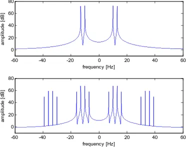
From the above equation we can see that there are several frequencies present at the output of Eq. (2). Additional terms to fundamental frequencies f1 and f2 can be divided into harmonic components 3f1 and 3f2 and
intermodulation products 2f1 ± f2 and f1 ± 2f2 as mentioned above. Similar operation with some amplitude scaling
is presented in Fig. 1, from which it can be seen that intermodulation terms are close to fundamental frequencies and thus probable to cause also self-interference in case of wideband or multicarrier system as DVB-H (Valkama et al., 2006).
-60 -40 -20 0 20 40 60
0 20 40 60 80 frequency [Hz] am pl it ude [ dB ]
-60 -40 -20 0 20 40 60
0 20 40 60 80 frequency [Hz] am pl it u de [ dB ]
Fig. 1. Distortion effects of 3rd order nonlinearity, generated 3rd harmonics and intermodulation products visible in the lower one.
On the other hand, out-of-band distortion caused by harmonic components visible in Fig. 1 can also be crucial in wideband receiver if adjacent channels aren’t totally filtered in the receiver front-end. One possible out-of-band distortion scenario is demonstrated in Fig. 2.
Fig. 2. Principle of out-of-band distortion generated by harmonic distortion.
In Fig. 2, the small signal in the right side of the upper picture at carrier frequency is the desired one and the left signal is the adjacent interfering signal. The distortion of desired signal is not considered in the figure. Harmonic terms visible in Fig. 2 are generated by 3rd, 5th and 7th order nonlinearities (Valkama et al., 2006).
Well known metrics of nonlinear behavior are third order Intercept Point (IP3) and 1dB Compression Point (CP). These values describe the saturation of characteristic curve. IP3 and 1dB CP are demonstrated in Fig. 3. Fundamental component can be approximated based on the level of third-order intermodulation distortion as in Eq. (3). x) 3 (IP 2 below
where x is the fundamental input level. IP3 and 1dB CP values will also be used to derive the nonlinearity implemented for the simulations (Renfors, 2008).
Fig. 3. IP3 and 1dB CP in relation to input signal level (Renfors, 2008)
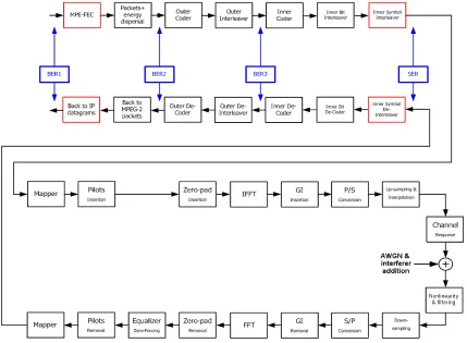
4. Simulation model
In order to study nonlinearity effects affecting DVB-H system, there is a need to simulate the transmission link first. The block diagram of the simulator model is given in Fig. 4. The properties of the simulation software are described in Table 1.
Table 1. DVB-H simulator properties
Modes 2K, 4K, and 8K
Modulations QPSK, 16-QAM, and 64-QAM Puncture rates 1/2, 2/3, 3/4, 5/6, 7/8
Cyclic prefix ratios 1/32, 1/16, 1/8, and 1/4 In-depth interleaving yes (2K & 4K) / no (8K)
Phase noise models PLL & Free-Running VCO with both white and flicker noise Channel models DVB-T F1 (Fixed) and DVB-T P1 (Portable)
Equalization: ZF using the pilots (scattered and continual)
Outputs SER; BER for Inner De-coding, Outer De-coding and FEC
To evaluate the nonlinearity effects on performance, some nonlinearity sources had to be added to the simulation chain. This was possible by adding a polynomial model in the simulator code that was making distortion to the signal in the channel corresponding to what would have happened with real nonlinear components. Important thing was also to choose a real nonlinear component with typical characteristics in this type of transmission link situation. The characteristics of the chosen components and their effects to the system in concern had to be figured out closely. Parameters reflecting these real components characteristics were then passed to mathematical nonlinearity model and converted into a polynomial. After that this polynomial could be used in the simulator to reflect realistic nonlinearity effects. After all of the modifications and additions to the simulator, it was finally ready for simulating different kinds of transmission scenarios.
5. Results and analysis
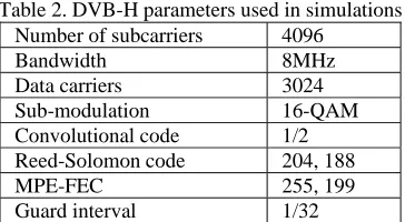
We have simulated the performance of DVB-H transmission link under receiver front-end nonlinearity. Most of the results are based on physical layer uncoded symbol error ratio, but also bit error ratios after error correction are considered. DVB-H system parameters used in simulations are presented in Table 2.
Table 2. DVB-H parameters used in simulations Number of subcarriers 4096
Bandwidth 8MHz
Data carriers 3024
Sub-modulation 16-QAM Convolutional code 1/2
Reed-Solomon code 204, 188
MPE-FEC 255, 199
Guard interval 1/32
The studies were done with DVB channel N+2 (second channel from desired one) and GSM900 uplink as interfering signals. Neighboring channel (N+2) can have maximum of +40dB power difference according to (Antoine, 2005). GSM interference is dimensioned according to maximum uplink transmission power of 2W. Taking coupling loss of 15dB between GSM transmitter and DVB-H receiver into account results in maximum interference power of
dBm 18 dB 15 dBm 33 coupling L transmit P GSM
P (4)
The setup is illustrated in Fig Interfering signals has been modeled with filtered Gaussian noise. Based on these values, some filtering and linearity requirements are evaluated (European Broadcasting Union, DVB-H Implementation Guideline, 2007).
5.1. Noise and Nonlinearity Models
Channel model used in simulation is additive white Gaussian noise (AWGN). In the receiver, thermal noise is added to signal and noise figure of 5dB is taken into account for receiver components. Thus added inband noise power on 8MHz bandwidth after filtering results in noise power defined by (Renfors, 2008)
dBm 100 W 13 10 * 0129 . 1 10 dB/ 5 10 MHz* 8 K* 290 * 23 3806503 . 1 kTBF noise
P (5)
For nonlinearity effects, the receiver front-end LNA is considered to be the source of distortion. The amplitude distortion in the system due to nonlinearity is modeled with polynomial equation which takes third and fifth order distortion into account. The coefficients are calculated from Output referred third order Intercept Point (OIP3). First Input referred third order Intercept Point (IIP3) was converted to OIP3 by
GAIN 3 IIP 3
OIP (6)
After that the terms re converted to normalized linear values by dB
10 GAIN/ 10 0
G (7)
0 *Z 3 10 * dBm 10 / 3 OIP 10 0 3
OIP (8)
0 *Z 3 10 * dBm 10 CP/ 10 0
P (9)
The coefficient values for amplitude to amplitude distortion polynomial were derived as follows s 4 s 6 c s 2 s 3 c s 1 c (s) AM/AM
F (10)
0 G 1
c (11)
0 3 *OIP 2 3 1 c 3
c (12)
1001 1 10 005 0 3 OIP 0 P 2 0 10 2 0 P 4 5 1 c 5
C . .
. (13)
where nominal impedance Z0=1Ω. The model has been obtained from Simulink general amplifier to model the
nonlinear behavior (The Mathworks, 2007). The values used to calculate coefficient values are obtained from the data sheet of LNA which is directed to GSM handsets and thus usable in this kind of evaluation. Most of the simulations were done with IIP3 = -11dBm, 1dB CP = -19dBm and GAIN = 16dB (ST Microelectronic, 2002).
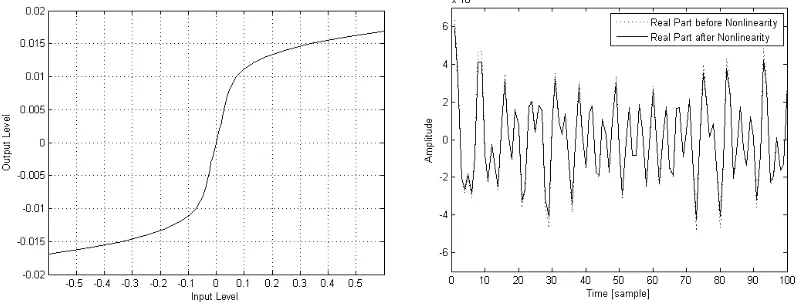
Amplifier nonlinearity – as an odd order polynomial – results in saturation of the voltage at certain level which can be seen from the characteristic curve of the model used in simulation, which is presented in Fig. 6a. Similar kind of behavior can also be seen from the simulated waveform in Fig. 6b where the highest amplitude values have disappeared.
Fig. 6. a. Characteristics curve of the nonlinear function applied in simulations. b. Time domain behavior of the real part (I-branch) of the
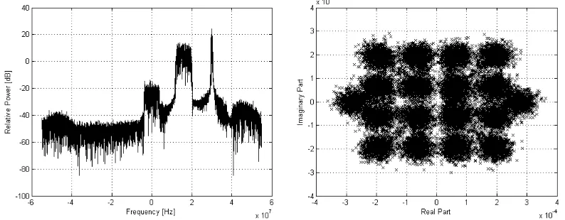
The severity of nonlinear behavior depends heavily on the level of the input signal. With input levels clearly below the value of 1dB CP, the system can be approximated to be linear and on the other hand with levels approaching the value of IIP3 the distortion raises fast (Renfors, 2008). The spectrum of the received signal remains mostly below the nonlinear region as can be seen in Fig. 7. High peak to average power ratio of an OFDM signal causes some saturation to happen when most of the signal has remained intact. Received symbol constellation of the same situation is shown in Fig. 7. It can also be seen from the constellation that some symbols values have suffered from nonlinear behavior.
Fig. 7. Signal spectrum and constellation after nonlinearity, desired signal power -70dBm and interferer relative powers +30dB.
When the signal power is made high, the effect of nonlinearity is even more obvious. This kind of situation is demonstrated in Fig. 8. From the spectral image of Fig. 8, the distortion can be seen as a rise of noise level, especially on third order intermodulation frequencies around -2MHz and 44MHz and also on third order harmonic frequency of -48MHz. In the constellation plot of Fig. 8, the interference can be seen as round Gaussian clouds due to the random nature of interfering signals. Two clouds on the sides of the constellation are additional pilot symbols.
Fig. 8. Signal spectrum and constellation after nonlinearity, desired signal power -60dBm and interferer relative powers +30dB
5.2. Minimum Received Signal Level
The minimum detectable signal level was studied with AWGN derived in Eq. (5). The power of the desired signal was varied and uncoded symbol error rate and bit error ratios after the coding stages were calculated. The results are given in Fig. 9 where the most interesting observation is that bit errors start to appear even after MPE-FEC stage that around input level of -85dBm to -90dBm. This is well in line with analytical sensitivity level for given sub-modulation and coding. Sensitivity level can be derived with
F N C noise P sens
P
dBm 90 dB 5 dB 6 . 9 dBm 16 .
105
(14)
where Pnoise is thermal noise power, C/N is carrier to noise ratio demanded for 16-QAM sub-modulation and
coding rate of 1/2 in Gaussian channel and F is the approximated noise figure for the receiver (European Broadcasting Union, DVB-H Implementation Guideline, 2007). The result also showed that BER3 and BER2 values were practically the same with only little variations. This rose doubts about the performance of Reed-Solomon coding block.
Fig. 9. Uncoded SER, BER after convolutional coding (BER3), BER after Reed-Solomon Coding (BER2) and BER after MPE-FEC (BER1)
as a function of received signal power
5.3. Maximum Received Signal Level
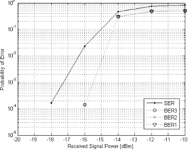
The saturation of the nonlinear system depends on the level of the input signal and thus the effects of different desired signal powers were studied. When the level reaches specified 1dB CP, the distortion starts to arise. This can also be seen from Fig. 10, where the results of the simulation are given.
With 1dB CP of -19dBm, errors start to appear with the signal levels of -18dBm and above. With lower power levels, the amplifier remains on linear region resulting in minimal distortion to signal. Though, coded BER values remain usable to as high levels as -16dBm or -15dBm which would be unusually high values for desired signal without interfering components. Maximum specified received level for desired DVB-H signal is stated to be -25dBm, which is well below the saturation range of the modeled amplifier (Antoine, 2005). The situation changes when presence of undesired signal is allowed also. In that kind of scenario, the overall power of signal entering the amplifier can’t be controlled inside the system in hand. Effect of this kind of interference is studied in the following chapters.
Fig. 10. Uncoded SER, BER after convolutional coding (BER3), BER after Reed-Solomon Coding (BER2) and BER after MPE-FEC (BER1) as a function of received signal power, nonlinearity with IIP3=-11dBm and 1dBCP=-19dBm
5.4. Tolerable Interference Level
system, the maximum power difference for adjacent channel (N+2) is specified to be +40dB when compared to desired one. In addition to that, GSM900 uplink channels are situated on nearby frequencies. Usually the case is such that DVB-H and GSM signals are both received and transmitted in mobile station. Thus the transmitted GSM signal can be coupled to receiver antenna with 10-20dB of coupling loss (European Broadcasting Union, DVB-H Implementation Guideline, 2007). These possible interference sources were modeled in simulations with filtered Gaussian noise signals to avoid some only signal structure dependant conclusions. Uncoded SER values gathered in the simulations are presented Fig. 11.
It can clearly be seen from the results that with very low received signal powers, SER values are noise dominated and the error ratio doesn’t drop to very low values even with mild interference. On contrary with higher desired signal levels, the changes in SER values are more rapid according to level of interference. Higher received power results in better signal to noise ratio and thus errors are rare with low interference levels. Though, when the interference gets more severe, there is rapid drop in the amount of properly detected symbol values. This is due to nonlinear behavior of the receiver when the overall received signal power is driven to saturation range.
Fig. 11. Uncoded symbol error ratio as a function of power of interfering signals relative to desired DVB-H power
5.5. Tolerable GSM Interference Level with Adjacent DVB-signal
Maximum level of adjacent DVB-H signals is specified in (European Broadcasting Union, DVB-H Implementation Guideline, 2007) and it is reasonable to expect the guidelines to be followed. In this sense we can expect the system to be able to deal with this kind of neighboring channels. On the other hand, GSM900 uplink is an extra-system signal and thus can’t be controlled in such way. Due to this fact it is interesting that how much extra-system interference received signal can handle in addition to well specified intra-system interference.
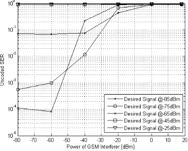
To study this behavior, power of GSM interferer is varied from -80dBm to +18dBm. The upper limit is derived from maximum transmit power of GSM mobile as was shown in Eq. (4). The neighboring channel DVB-H interferer level is kept at constant power level of +40dB in relation to the desired one. The resulting SER values for different setups are shown in Fig. 12.
From the results above, it can be seen that the low desired signal power levels are noise dominated. In contrary with highest power values, overall power is so high, that the desired signal is lost due to nonlinear behavior. With levels in between previous ones, the ratio of correct symbol detection is kept on reasonable level for GSM interference powers below -40dBm and -50dBm.
Based on these observations, the filtering requirements for the GSM900 uplink band can be derived for DVB-H receiver. Assuming that GSM power entering the receiver should be less than -50dBm, we end up to filter attenuation requirement of
dB 68 dBm) 50 ( dBm 18 tolerable P GSM P filter
L (15)
which is relatively high demand for Radio Frequency (RF) filter with high selectivity. 5.6. Needed Receiver Linearity in Worst Case GSM Interference
Some GSM interference will be received also in DVB-H system due to limited range of RF filter attenuation, if the full GSM900 uplink power is utilized. Assuming typical RF filter attenuation of 60dB (Renfors, 2008) – even which could be challenging to reach due to proximity of the signal bands - the remaining interference power would be
dBm 42 dB 60 dBm 18 filter L GSM P ed GSM,filter
P (16)
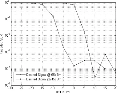
This kind of scenario is then simulated with the adjacent DVB-channel with relative power of +40dB to desired one. The purpose of this is to derive linearity requirements for the receiver front-end in worst case interference scenario. The results are given in Fig. 13.
Fig. 13. Uncoded symbol error ratio as a function of input referred third order intercept point (IIP3) with DVB interferer power being +40dB
to desired signal and GSM interferer constant at -42dBm
It can be seen that even with the optimal level of desired signal power, IIP3 value of the receiver should be more than -10dBm. This should contain the cascaded values of used components. Typical setup could be for example LNA, mixer and analog-to-digital converter. Based on the values obtained from (ST Microelectronic, 2002), this kind of requirement is challenging even for the sole LNA. Amplifiers with higher linearity values are of course available but especially in consumer products, such as mobile phones, there is a drive towards cheaper analog components. Thus it can be said that this kind of scenario will be challenging for front-end design and DVB-H reception under GSM900 uplink interference.
6. Conclusion
According to results obtained during the analysis, GSM900 uplink interference is an issue in mobile receiver designed for DVB-H transmissions. The scenario is especially challenging because of the immediate proximity of system frequency bands. The effect of this is that it makes the design of an RF filter with enough attenuation challenging in case of such a narrow transmission band.
According to the simulation results, the worst case interference scenario with 60dB RF filter attenuation would result in approximately 10% of uncoded SER. Despite the fact that this is quite high value, the error coding applied in simulations can lower the ratio considerably when considering BER values after decoding. On the other hand, it should be noted that one DVB-H frame with the applied settings consists of almost two million bits leading into strict demand for BER in order to receive whole non-erroneous frames.
References
[1] Antoine, P. et al. (2005): "A Direct Conversion Receiver for DVB-H," IEEE Journal of Solid State Circuits, vol. 40, no. 12, pp. 2536-2546.
[2] European Broadcasting Union, DVB (2004): "Digital Video Broadcasting (DVB); Framing structure, channel coding and modulation for digital terrestrial television," The European Telecommunications Standards Institute, ETSI EN 300 744.
[3] European Broadcasting Union, DVB-H (2004): "Digital Video Broadcasting (DVB) (2004): Transmission System for Handheld Terminals (DVB-H)," The European Telecommunications Standards Institute, ETSI EN 302 304.
[4] European Broadcasting Union, DVB-H Fact-Sheet (2008): DVB-H Fact Sheet [Online]. http://www.dvb-h.org/PDF/dvb-h-fact-sheet.0409.pdf
[5] European Broadcasting Union, DVB-H Implementation Guidelines (2007): DVB-H Implementation Guidelines. [Online]. http://dvb-h.org/PDF/a092r2.tm2977r11.dTR102377.V1.3.1.DVB-H_impl_guide.pdf.
[6] Kornfeld, M. and Daoud K. (2008): "The DVB-H mobile broadcast standard [standards in a nutshell]," IEEE Signal Processing Magazine, vol. 25, no. 4, pp. 118-122.
[7] Renfors, M.(2008): "Receiver Architectures," Tampere University of Technology, Lecture Slides.
[8] ST Microelectronic. (2002): 900MHz Three Gain Level LNA. [Online]. http://www.datasheetcatalog.org/datasheet/stmicroelectronics/7666.pdf
[9] The Mathworks. (2007): Simulink [Online]. http://www.mathworks.com/products/simulink/.