AN ALGORITHM FOR RETRIEVAL OF
AEROSOL PROPERTIES FROM LIDAR
OBSERVATIONS
Y. BHAVANI KUMAR, Member IEEE
Project Leader, LIDAR project, National Atmospheric Research Laboratory (NARL) Gadanki-517112, Andhra Pradesh, India
S. VIJAYA KUMAR VARMA Professor, Department of Mathematics Sri Venkateswara University, Tirupati – 517502, India.
Abstract:
A mathematical method of computing aerosol properties from the micro pulse lidar observations is described in this paper. The developed mathematical inversion algorithm has been tested on the indigenously developed micro pulse lidar data and successfully derived height profiles of aerosol backscatter in the lower atmosphere. Observation results in terms of aerosol backscattering coefficient are presented and discussed.
Keywords: Lidar inversion, micro pulse lidar, aerosol backscattering coefficient, mathematical algorithm
[1] Introduction
Aerosols are tiny particles suspended in the atmosphere. They exist either in solid or liquid phase. Aerosol particles are injected into the atmosphere by natural and anthropogenic sources. The natural sources of aerosol particles comprise pollen from flowers, sea salt spray, dust blowing over the desert and ash from wildfires and volcanoes. The anthropogenic (man made) aerosol sources include particles from factory smoke, auto emissions and slash-and-burn agricultural works.
Aerosol measurements can be performed using passive and active remote sensing methods. The passive remote sensing methods are capable of providing the aerosol load on wide spectral ranges, but they offer the columnar integrated measurements. On the contrary, lidar measurements are valuable and provide information on the vertical profiles of aerosol properties [Bhavani Kumar (2009)]. The altitude of aerosol particles is important, because particles at lower altitudes are likely to be washed out of the atmosphere by rain, and will not have a long-term effect on the climate. However, those that achieve a higher altitude are likely to remain airborne much longer and will travel greater distances from the point of origin. The long-range transport of aerosols influences the climate and effects the environment [Ramanathan et al (2001)].
Kumar (2006)] that employs a new approach of high pulse repetition rate with low pulse power transmitter. A number of articles have reported the application of portable lidar to the environmental studies [Hegde et al
(2009); Badarinath et al (2009); Bhavani Kumar and Purusotham (2010)].
[2] Portable lidar system
The portable lidar system [Bhavani Kumar (2006)] discussed in this study was indigenously developed at the National Atmospheric Research Laboratory (NARL), an autonomous institution under Department of Space, located at Gadanki (13.5N, 79.2E, 375 m AMSL), a rural site near Tirupati city in Andhra Pradesh. The lidar system was developed under a project titled “Boundary Layer Lidar (BLL)”. The lidar system employs micro pulse technique and its technical configuration is quite different from the micro pulse lidar [Spinhirne (1993)]. The lidar system employs a diode pumped Nd:YAG laser that operates at its second harmonic wavelength (532 nm). The output pulse energy is set at 10 J with a repetition rate of 2.5 kHz. The lidar system uses a 150 mm diameter Cassegrain telescope for collecting the laser-backscattered returns from the atmosphere. The lidar employs photon-counting detector electronics, a fast discriminator (300 MHz) and a PC-based multi channel scalar (MCS) add-on card.
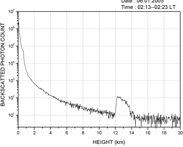
Fig. 1 Basic photon count profile from the portable lidar system obtained at lidar site during midnight hours between 02:13 and 02:23 LT
on 6 January 2005. A strong scattering layer observed at heights between 12 and 14 indicates the occurrence of high altitude cloud over
the lidar site during the observational period.
logarithmic scale and shown up to 20 km height. The signal profile was collected during midnight hours between 02:13 and 02:23 local time (LT) on 6 January 2005. The photon count profile corresponds to a time integration of 10 minutes. A layer of strong scattering is clearly seen in the upper troposphere at heights between 12 and 14 km, which corresponds to the occurrence of high altitude cloud over the lidar site during the period of observation. The nonzero count level observed beyond the signal range is caused primarily due to the background light.
[3] Mathematical algorithm
The retrieval of aerosol backscatter from lidar returns depend on the attenuation of the signal on its path through the atmosphere. The functional expression [Collis (1969)] that relates outgoing laser energy (E0) and the backscattered signal P (z) is given as
b T P z T z z z O KE z
P( ) ( ) ( ) 2( )
2 0
(1)where E0 is the laser pulse energy, K the lidar system constant, O(z) the overlap function (for portable lidar system, O(z)=1 for heights more than 200 m above ground level). In the atmosphere two types of optical scattering takes place: scattering by the air molecules and solid particles or liquid droplets suspended in the air. The received laser radiation measured by lidar is proportional to the effective backscattering from particles and molecules present in the atmosphere.
In Eq. (1), the term T (z) represents the total volume backscatter coefficient, which is the sum of
backscatter from air molecules m (z) and particles a (z) interacted by the laser photons. The term T (z) refers
to the atmospheric transmittance for the laser photons traveling from ground to a given distance
z
in the atmosphere and back to the source. This is usually represented as
z
T
z
dz
z
T
0 2]
)
(
2
exp[
)
(
(2)Where the term T (z) is the total volume extinction coefficient, given as the sum of the integrated attenuation
due to air molecules m (z) and particles a (z).
For any lidar system, Eq. (1) can be modified and shown as b T P z z T z C z
P 2
2 ) ( ) ( )
(
(3)where C is the calibration constant and can be extracted from the lidar signal P(zc) at a reference calibration
range zc by
0 2 2 ) ( ) ( ) ( ) ( E z T z R z z P z C c c m c c
. (4)
Here R (zc) is the atmospheric mixing ratio at range zc. In the present study, the calibration height range is
considered at heights between 7 and 10 km. Since the signal counts in this height range are small, several range bins are averaged to obtain mean calibration constant. In Eq. (3), the term Pb relates to the sky
Since the lidar equation has strong dependence on path loss (range square loss) due to the telescope etendue, Eq. (3) is often reduced to a form
z
T T
b
z
z
dz
C
z
P
z
P
z
0 2 ']
)
(
2
exp[
)
(
]
)
(
[
)
(
(5)where the term '(z) is known as attenuated backscatter coefficient. By applying natural logarithm and differentiating both sides of Eq. (5), one obtains
{ln[
(
)]}
{ln[
(
)]}
2
(
)
'
z
dz
z
d
dz
z
d
T T
. (6)This equation is a function two variables, namely T (z) and T (z). It cannot be solved unless a relation between
extinction and backscattering coefficient is assumed. The relation is termed as lidar ratio (LR). For molecular (Rayleigh) atmosphere, the extinction to backscatter ratio (LRm) is constant and fixed at 8/3. The molecular
backscatter cross-section and Rayleigh extinction data can be obtained by using formulation given in literature [Bodhaine et al (1999)]. The height profile of molecular components such as m(z) and m(z) can be computed
from pressure P(z) and temperature T(z) data given by meteorological radiosondes or by using the standard model atmosphere data from the following relations:
)
(
)
(
)
(
)
7
6
(
)
2
(
)
3
6
(
)
1
(
9
)
(
0 0 2 2 2 4 2 2 2z
T
z
P
P
T
N
n
N
n
z
s air s airm
(7))
(
)
(
)
(
)
7
6
(
)
2
(
)
3
6
(
)
1
(
24
)
(
0 0 2 2 2 4 2 2 3z
T
z
P
P
T
N
n
N
n
z
s air s airm
(8)where nair represents the refractive index of air (nair =1.00027824 at 530 nm),
indicates the airdepolarization (0.00376) [Behrendt and Nakamura (2002)] at the operating wavelength and corresponding to King’s factor of 1.049 at 530 nm, and the factor Ns = 2.547×1025 m-3 gives the molecular number density for
the standard atmospheric pressure (P0 = 1013.25 mbar) and temperature (T0 = 288.15 K) conditions at the ground respectively. In the present study, the above empirical relations have been used in a computer code for deriving the molecular profiles, such as backscattering coefficient m(z) and extinction coefficient m(z), from
the atmospheric pressure and temperature data corresponding to the geographical coordinates of the lidar site given by the standard atmosphere CIRA-86 [Fleming et al (1988)].
However, the determination of aerosol extinction and backscatter (LRa) is not straightforward as in the
case of air molecules, because their extinction and backscatter depends on the size distribution and refractive indices of the particles present in the atmosphere. Generally, atmospheric aerosol/particles can be represented as homogeneous spheres and Mie Theory can predict their optical properties as functions of size distribution and refractive index. Several investigators have calculated LRa values for tropospheric aerosols from size and
chemical information either by measurement or by calculation. However, numerous evidences [Ackerman (1997); Doherty et al (1999)] indicate that lower LRa -values (less than 30) are associated with cases where the
coarse mode is more dominant and that higher LRa-values (above 40) are associated with cases where
pollution-derived accumulation -mode particles are more prominent. As the lidar site is located in a non-polluted land-locked rural region, a representative value of 40 has been used in the present study as LRa
Once the lidar ratio for aerosol is assumed, the application of two-component signal inversion to Eq. (6) allows determination of a. Since this equation is a Ricatti type one (Bernoulli’s form), the differential
equation of first order and its solutions are given as
z z a m a c dz term z LR term term z z z 1 ' 2 1 ' ) ( 2 ) ( ) ( ) ( . (9)
Here
zz m m a c dz z LR LR
term1 exp 2( )
( ) (10)and ) ( ) ( ) ( ' 2 C m C a C z z z term
. (11)
This solution is called the “forward” solution, since the proposed solution is based on a reference calibration point for the aerosol scattering coefficient and extinction -to-backscatter ratio at a distance less than the retrieval distance. This was convenient when auxiliary measurement of the light scattering coefficient (such as with an integrated nephelometer) were available in the near field. However, it has been pointed out [Klett (1981)] that the solution of Eq. (9) could become unstable for cases of high extinction and would diverge with increased altitude, z. Thus, a “backward” solution is generally more preferable, where the known calibration position was beyond the region where the retrieval is to be performed. To facilitate this, reordering of the orders of integration and the change of sign in the denominator are required in Eq. (9). This makes the solution more stable, provided the aerosol scattering coefficient in the calibration point can be estimated properly.
[4] Experimental results
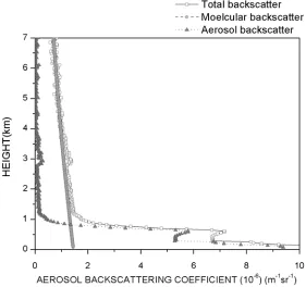
Using the backward integration method, a computer code has been developed for deriving the aerosol scattering coefficient from the portable lidar data. The developed code initializes from the mean calibration range bin with an indicated value of aerosol lidar ratio and an assumed value of aerosol scattering coefficient at the top as input parameters. Fig. 2 shows the derived height profiles of the total, molecular and aerosol backscattering coefficient from lidar returns using the developed algorithm. However, the assumed value of aerosol backscatter coefficient at the calibration height plays an important role in the retrieval of aerosol profile and imposes an error in the derived aerosol backscatter. Hence, the developed lidar algorithm has been verified for different values of aerosol backscattering coefficient at the calibration point to check the sensitivity of the derived aerosol backscatter coefficient profile and to estimate the error introduced in the derived aerosol-backscattering coefficient. As a result, it turns out that the error in the aerosol-backscattering coefficient is in the range of 5 to 10% for a variation of assumed aerosol input value by an order of 2. Moreover, the developed algorithm has also been verified for different theoretical values of lidar ratio (LRa)
and tested for different calibration heights. The derivation of the aerosol backscatter has shown less dependence on the choice of LRa and on the altitude of calibration height chosen. The range of variation of in
Fig. 2 Height profiles of aerosol backscatter derived from lidar. The profiles show the total, molecular and aerosol backscatter profiles
covering 7 km in the lower troposphere.
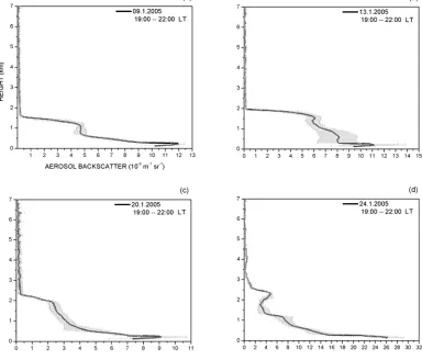
Fig. 3 gives the averaged profiles of aerosol backscatter derived on selective days plotted along with the variability in the data. It is noticed from these profiles that the standard deviation is high in the boundary layer than in the free troposphere. The most regular feature of all profiles shown is the presence of a large particle layer in the lowermost troposphere. This layer most likely corresponds to the local mixing layer (ML). During the period of experiment on the vertical extent of aerosol mixing, the top height of ML varied between 1 and 3 km. The increase in the vertical extent of maximum aerosol amount could be the result of the increase in surface temperature during daytime, which pushes the vertical extent of the boundary layer up and gives more vertical space for aerosols to mix and move through advection during nighttime. The increase in the vertical extent of the boundary layer thus results in diluting the surface level aerosol concentration. The height of the nighttime ML is an important parameter for the characterization of the air exchange with the free troposphere and for an estimation of the aerosol dilution within the boundary layer [Stull (1988)].
5. Conclusion
Fig. 3 Height profiles of mean aerosol backscatter observed on selected days to show the aerosol backscatter variability during the period
of observation. The variability in the aerosol backscatter is shown as shaded lines about the mean aerosol profile.
Acknowledgements
One of the authors, Dr. Y.Bhavani Kumar, would like to thank the National Atmospheric Research Laboratory (NARL) and Atmospheric Science Programme (ASP) office of Department of Space, Government of India for funding the project “BLL development and studies”.
References
[1] Bhavani Kumar, Y (2009): Development of LIDAR techniques for environmental remote sensing and mathematical analysis of
atmospheric data, Doctoral thesis submitted to Sri Venkateswara University, Tirupati (Awarded).
[2] Ramanathan, V et al., (2001): Indian Ocean experiment: An integrated analysis of the climate forcing and effects of the great
Indo-Asian haze. Journal of Geophysical Research, 106(D22), pp 28371–28398.
[3] Reagan, J.A; McCormick, M.P; Spinhirne, J.D (1989): Lidar sensing of aerosols and clouds in the troposphere and
stratosphere. Proc. IEEE. 77, pp. 433-448.
[4] Bhavani Kumar Y (2006): Portable lidar system for atmospheric boundary layer (ABL) measurements, Optical Engineering,
45: pp 076201-5.
[5] Hegde, P.P; Pant, P; Bhavani Kumar (2009): An integrated analysis of lidar observations in association with optical properties
[6] Badarinath, K.V.S; Anu Rani Sharma; Shailesh Kumar Kharol (2009): LIDAR Observations of Aerosol Properties Over
Tropical Urban Region—A Case Study During a Low-Pressure System Over Bay of Bengal, IEEE Geoscience and Remote
sensing, 6(4),pp 807-811.
[7] Bhavani Kumar, Y; Purusotham. S (2010): Mathematical algorithms for determination of mixed layer height from laser radar
signals, International Journal of Computer Science and Engineering, Vo.2 (6), 2059-2063.
[8] Spinhirne, J.D (1993): Micro pulse lidar, IEEE Transactions on Geoscience Remote Sensing, 31, pp 48-54.
[9] Collis, R.T.H (1969): Lidar for routine meteorological observations, Bulletin of American Meteorological Society, 50 pp 688–694.
[10] Bodhaine, B.A.; Wood, N.B.; Dutton, E.G; Slusser, J.R (1999): On Rayleigh optical depth calculations, Journal of Atmosphere
and Ocean technology, 16, pp1854–1861.
[11] Behrnedt, A; Nakamura, T (2002): Calculation of the calibration constant of polarization lidar and its dependence of polarization
lidar and its dependence on atmospheric temperature, Opt. Express,10, 805-817.
[12] Fleming, E.L; Chandra, S; Shoeberl, M.R; Barnett, J.J (1988) Monthly mean global climatology of temperature, wind,
geopotential height and pressure for 0-120 km, National Aeronautics and Space Administration, Technical Memorandum
Washington.
[13] Ackerman, J (1997): The extinction to backscatter ratio of tropospheric aerosol: A numerical study, Journal of Atmosphere and
Ocean technology, 15, pp 1043-1050.
[14] Doherty, S.; Anderson, T.L; Charlson, R.J (1999): Measurement of the lidar ratio for atmospheric aerosols using a 180
backscatter nephelometer, Applied Optics, 38, pp. 1823-1832.