EFFECT OF DISTANCE MEASURES ON TRANSFORM BASED IMAGE CLASSIFICATION

(1)

EFFECT OF DISTANCE MEASURES ON

TRANSFORM BASED IMAGE

CLASSIFICATION

H. B. KEKRE

Sr. Professor,

MPSTME, NMIMS University, Vileparle(w) Mumbai-56, INDIA

[email protected]

TANUJA K. SARODE

Associate Professor,

Thadomal Shahani Engineering College, Bandra(W), Mumbai-50, INDIA

[email protected]

JAGRUTI K. SAVE

Ph.D. Research Scholar, MPSTME, NMIMS University,

Associate Professor,

Fr. CRCE, Bandra(W), Mumbai-50, INDIA [email protected]

Abstract :

Due to rapid growth of multimedia databases, there is a need to classify and organize these databases. Classification of image database is a computational procedure that sorts images into groups (classes) according to their similarities. Many algorithms have been developed for this purpose. Measuring similarity or distance between two feature vectors is a key step in all these algorithms. Choosing the right distance measure for a given database is a biggest challenge. In this paper, we study various distance measures and their effect on transform based image classification methods. The paper presents a comparison between different distance measures for various sizes of feature vectors. 8 classes of images from the Wang database are used to carry out the experiments. The experimental results and detailed analysis are presented.

Keywords: Classification; Similarity Measures; Image Transforms; Feature Vector; Nearest Neighbor Classifier; Minkowski Distances; Cosine Correlation Similarity;.

1. Introduction

(2)

its significance; in section 3, we present the classification algorithm; Section 4 gives the results followed by conclusion and future work.

2. Distance Measures

Many distance measures have been proposed in literature for image classification [14]. In this section we briefly elaborate six commonly used distance measures. An important family of distance measures is formed by Minkowski distances [15] [16]. If P = (P1,P2,…,Pn) and Q = (Q1,Q2,…,Qn) are two feature vectors, then the Minkowski distance of order p between them is given by Eq.1.





p

n

i

p i i

Mink

P

Q

P

Q

D









1

,

(1)

The L1 (1-norm) Minkowski distance is the Manhattan distance and the L2 distance is the Euclidean distance. When p goes to infinite, we get Chebyshev distance.

2.1. Euclidean Distance

Euclidean distance is a standard metric for geometrical problems. Euclid stated that the shortest distance between two points is a length of a straight line joining those two points and thus the Eq.2 is predominantly known as Euclidean distance. It is the ordinary distance between two points and can be easily measured with a ruler in two or three-dimensional space. Euclidean distance is widely used in K nearest neighbor classification problems [17].





_







n i i i

Euc

P

Q

P

Q

D

1

2

,

(2)

2.2. Manhattan Distance

It is a distance between two points measured along axes at right angles. It is also known as rectilinear distance or city block distance. It is given in Eq.3. It requires less computation than many other distance metrics.





_

   n i i i

Man P Q P Q

D

1

, (3)

2.3. Chebyshev Distance

In mathematics, Chebyshev distance, Maximum metric, is a metric defined on a vector space where the distance between two vectors is the greatest of their differences along any coordinate dimension. It is named after Pafnuty Chebyshev. It is as given in Eq.4.





_i i i

Cheb

P

Q

P

Q

D

,



max



(4)

It is also known as chessboard distance, since in the game of chess the minimum number of moves needed by a king to go from one square on a chessboard to another equals the Chebyshev distance between the centers of the squares.

2.4. BrayCurtis Distance

The Bray–Curtis dissimilarity, named after J. Roger Bray and John T. Curtis [18] is a statistic used to quantify the compositional dissimilarity between two different sites, based on counts at each site. The distance based on Bray-Curtis dissimilarity is given in Eq.5. It is widely used in ecology, biology and environmental science. It is also known as Sorensen distance. It views the space as grid similar to the city block distance.











 







_n i i i n i i i BC

Q

P

Q

P

Q

P

D

1 1

,

₍₅₎

2.5. Canberra Distance

(3)

that the absolute difference between the variables of the two objects is divided by the sum of the absolute variable values prior to summing.





_

_

_









n

i i i

i i

Can

_P

_Q

Q

P

Q

P

D

1

,

(6)

2.6. Cosine Correlation Distancee

Cosine similarity is a measure of similarity between two vectors by measuring the cosine of the angle between them. As the angle between the vectors shortens, the cosine angle approaches 1, meaning that the two vectors are getting closer, meaning that the similarity of images represented by the vectors increases. This distance is often used to compare documents in text mining [20] and given in Eq.7







    n i i n i i n i i i Corr Q P Q P Q P D 1 2 1 2 1

,

(7)

Euclidean distance varies with variation in the scale of the feature vector but cosine correlation distance is invariant to the scale transformation.

3. Classification Algorithm

The image database (total 280 images) is divided into a training set (40 images that is 5 images from each class) and a testing set (240 images that is 30 images from each class). The feature vector of each training/testing image is generated as given below.

3.1. Generation of feature vector

(1)For each color image, generate its three color (R, G, and B) planes.

(2)one Apply following transforms on columns of an image for all three planes. (i) Discrete Fourier Transform (DFT)

(ii) Discrete Cosine Transform (DCT) (iii) Discrete Sine Transform (DST) (iv) Hartley Transform [21] (v) Walsh Transform[22] (vi) Kekre Transform[23]

(3)Calculate row mean vector of each column transformed image for three planes [24][25].

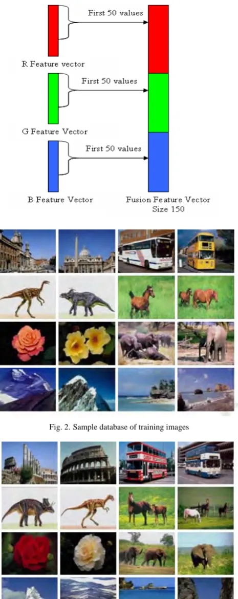
(4) Make a feature vector by fusing the row mean vectors of R, G, and B plane as shown in Fig.1. Different values of feature vector size like 150 (50R + 50G + 50B), 225 (75R + 75G + 75B) etc. are also considered to generate feature vectors.

3.2. Classification

Nearest neighbor classifier algorithm is used [26]. Similarity between training feature vector and testing feature vector is calculated using the different distance formulae. Minimum distance indicates the most similar training image for that testing image and the corresponding class. We have also considered another training set where each feature vector is the average of feature vectors of all training images of a particular class.

4. Results

(4)

Fig. 1. Fusion of three feature vectors

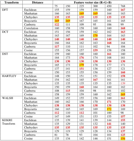
Fig. 2.Sample database of training images

(5)

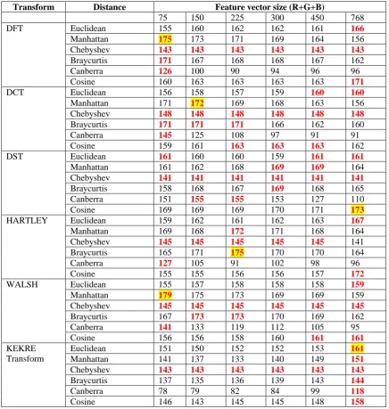
Table 1. Number of correctly classified images (out of 240) for various distance measures for different feature vector sizes Training set: Feature vectors of 5 images from each class.

Transform Distance Feature vector size (R+G+B)

75 150 225 300 450 768

DFT Euclidean 155 159 159 159 160 167

Manhattan 166 163 169 169 164 163

Chebyshev 135 135 135 135 135 135

Braycurtis 169 169 167 165 161 165

Canberra 122 111 109 95 106 99

Correlation 160 158 158 160 160 168

DCT Euclidean 151 156 159 162 162 163

Manhattan 163 167 169 170 164 163

Chebyshev 140 140 140 140 140 140

Braycurtis 166 164 162 163 168 164

Canberra 117 110 111 102 94 104

Cosine 155 156 157 159 158 158

DST Euclidean 159 160 160 160 161 160

Manhattan 164 173 176 174 168 161

Chebyshev 130 130 130 130 130 130

Braycurtis 165 173 179 178 177 171

Canberra 137 141 151 136 127 121

Cosine 150 153 155 156 159 160

HARTLEY Euclidean 148 150 151 151 152 158

Manhattan 154 162 165 167 161 161

Chebyshev 135 135 135 135 135 139

Braycurtis 150 159 168 164 160 162

Canberra 108 115 104 98 101 102

Cosine 158 159 159 160 162 169

WALSH Euclidean 149 152 155 156 160 161

Manhattan 160 162 166 170 171 170

Chebyshev 138 138 138 138 138 138

Braycurtis 166 165 165 169 172 169

Canberra 112 110 112 101 100 98

Cosine 147 149 151 153 155 157

KEKRE Transform

Euclidean 135 139 141 139 144 155

Manhattan 135 129 131 132 141 140

Chebyshev 135 135 135 135 135 135

Braycurtis 129 119 129 128 134 137

Canberra 81 78 93 104 101 125

Cosine 135 134 142 146 151 156

Note: For each distance, highest number of correctly classified images is shown in red color. For each transform, highest number of correctly classified images is shown in red color with yellow background.

Table 2. Highest Number of correctly classified images (out of 240) for each transform Training set: Feature vectors of 5 images from each class

TRANSFORM Highest Number of Correctly Classified Images(out of 240)

Distance Measure Feature Vector size

DFT 169 Manhattan 225&300

Bray-Curtis 75&150

DCT 170 Manhattan 300

DST 179 Bray-Curtis 225

HARTLEY 169 Cosine 768

WALSH 172 Bray-Curtis 450

(6)

Table 3 Number of correctly classified images (out of 240) for various distance measures for different feature vector sizes Training set: Average of feature vectors of 5 images from each class.

Transform Distance Feature vector size (R+G+B)

75 150 225 300 450 768

DFT Euclidean 155 160 162 162 161 166

Manhattan 175 173 171 169 164 156

Chebyshev 143 143 143 143 143 143

Braycurtis 171 167 168 168 167 162

Canberra 126 100 90 94 96 96

Cosine 160 163 163 163 163 171

DCT Euclidean 156 158 157 159 160 160

Manhattan 171 172 169 168 163 156

Chebyshev 148 148 148 148 148 148

Braycurtis 171 171 171 166 162 160

Canberra 145 125 108 97 91 91

Cosine 159 161 163 163 163 162

DST Euclidean 161 160 160 159 161 161

Manhattan 161 162 168 169 169 164

Chebyshev 141 141 141 141 141 141

Braycurtis 158 168 167 169 168 165

Canberra 151 155 155 153 127 110

Cosine 169 169 169 170 171 173

HARTLEY Euclidean 159 162 161 162 163 167

Manhattan 169 168 172 171 168 164

Chebyshev 145 145 145 145 145 141

Braycurtis 165 171 175 170 170 164

Canberra 127 105 91 102 98 96

Cosine 155 155 156 156 157 172

WALSH Euclidean 155 157 158 158 158 159

Manhattan 179 175 173 169 169 159

Chebyshev 145 145 145 145 145 145

Braycurtis 167 173 173 170 169 162

Canberra 141 133 119 112 105 95

Cosine 156 156 158 160 161 161

KEKRE Transform

Euclidean 151 150 152 152 153 161

Manhattan 141 137 133 140 149 151

Chebyshev 143 143 143 143 143 143

Braycurtis 137 135 136 139 143 144

Canberra 78 79 82 84 99 118

Cosine 146 143 145 145 148 158

Note: For each distance, highest number of correctly classified images is shown in red color. For each transform, highest number of correctly classified images is shown in red color with yellow background.

Table 4. Highest Number of correctly classified images (out of 240) for each transform Training set: : Average of feature vectors of 5 images from each class

TRANSFORM Highest Number of

Correctly Classified Images(out of 240)

Distance Measure Feature Vector size

DFT 175 Manhattan 75

DCT 172 Manhattan 150

DST 173 Cosine 768

HARTLEY 175 Bray-Curtis 225

WALSH 179 Manhattan 75

(7)

4.1. Observations

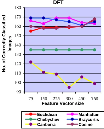
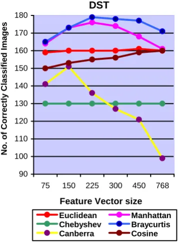
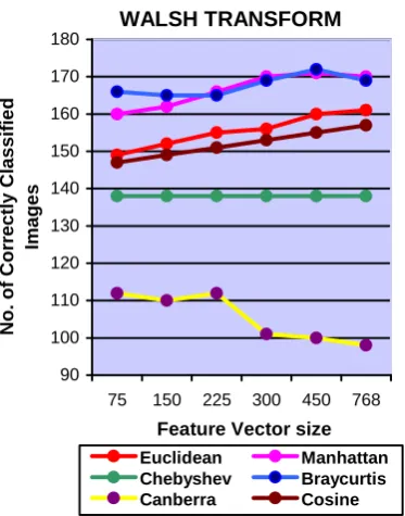
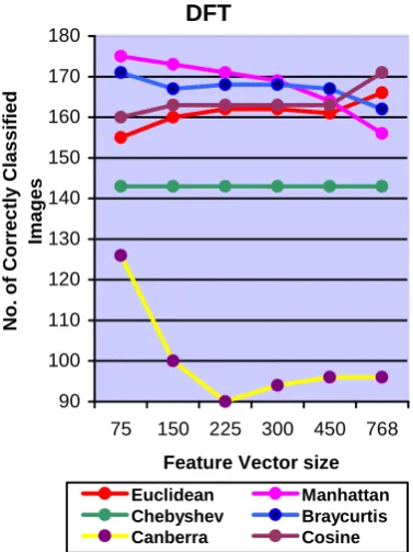
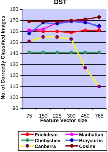
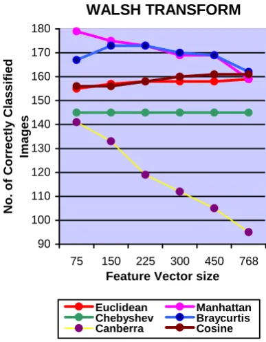
Euclidean and Cosine similarity gives better performance when we select larger size of feature vector. Manhattan, Bray Curtis and Canberra distances give good performance for comparatively smaller size of feature vectors in DFT, DCT, DST, WALSH and HARTLEY. In KEKRE transform all distances give better performance for large size of feature vector. Chebyshev distance remains almost constant with different sizes of feature vectors. Canberra distance gives worst performance when compared with other distances. Figure 4 to Figure 15 shows the number of correctly classified images for different transforms. These figures describe the performance of different distances for different feature vector size for particular transform. For Figure 4 to Figure 9, training set is the feature vectors of 5 images from each class. For Figure 10 to Figure 15, the training set is the average of feature vectors of 5 images from each class.

DFT

90 100 110 120 130 140 150 160 170 180

75 150 225 300 450 768

Feature Vector size

No.

of

Cor

rect

ly Cl

ass

if

ied

Im

ages

Euclidean Manhattan Chebyshev Braycurtis Canberra Cosine

(8)

DCT

90 100 110 120 130 140 150 160 170 180

75 150 225 300 450 768

No.

of

Cor

rect

ly Cl

assi

fi

e

d I

m

ages

Fig. 5 Performance of distances for DCT

DST

90 100 110 120 130 140 150 160 170 180

75 150 225 300 450 768

N

o

. of

C

o

rr

ect

ly C

lassif

ied I

m

ages

(9)

HARTLEY TRANSFORM

90 100 110 120 130 140 150 160 170 180

75 150 225 300 450 768

N

o

. o

f C

o

rrec

tly C

lassified

Im

ag

es

Fig. 7 Performance of distances for HARTLEY

WALSH TRANSFORM

90 100 110 120 130 140 150 160 170 180

75 150 225 300 450 768

No.

of

Cor

rect

ly Cl

assi

fi

e

d

Im

ages

(10)

KEKRE TRANSFORM

70 80 90 100 110 120 130 140 150 160 170 180

75 150 225 300 450 768

No.

of

Co

rr

ect

ly Cl

assi

fi

ed I

m

ages

Fig. 9 Performance of distances for KEKRE Transform

DFT

90 100 110 120 130 140 150 160 170 180

75 150 225 300 450 768

No.

of

Cor

rec

tl

y Cl

assi

fi

ed

Im

ages

(11)

DCT

90 100 110 120 130 140 150 160 170 180

75 150 225 300 450 768

N

o

. o

f C

o

rrectly C

lassified

Im

ag

es

Fig. 11 Performance of distances for DCT Transform for average feature vector

DST

90 100 110 120 130 140 150 160 170 180

75 150 225 300 450 768 Feature Vector size

N

o

. o

f C

o

rr

ectly C

lassified

Im

ag

e

s

(12)

HARTLEY TRANSFORM

90 100 110 120 130 140 150 160 170 180

75 150 225 300 450 768 Feature Vector size

N

o

. of

C

o

rr

ect

ly C

lassif

ied Ima

g

es

Fig. 13 Performance of distances for HARTLEY TRANSFORM for average feature vector

WALSH TRANSFORM

90 100 110 120 130 140 150 160 170 180

75 150 225 300 450 768

N

o. of C

or

rectly C

lassified

Images

(13)

KEKRE TRANSFORM

70 80 90 100 110 120 130 140 150 160 170 180

75 150 225 300 450 768

N

o. of C

or

rectly C

lassified Im

ages

Fig. 15 Performance of distances for KEKRE TRANSFORM for average feature vector

5. Conclusions

This paper presents a comparative study of the different distance/similarity measure criteria in classification of images. The feature vector is generated from an image column transform. The performance of various distance criteria such as Minkowski Distances (Euclidean, Manhattan, Chebyshev), BrayCurtis, Canberra and Cosine similarity is tested thoroughly using different transforms (DFT, DCT, DST, HARTLEY, WALSH and KEKRE); on different sizes of feature vectors (75, 150, 225, 300, 450 and 768) for two training sets (feature vectors, average of feature vectors). From the results it can be concluded that the training set containing average of feature vectors, gives equally good results and since they are small in numbers (only 1 training feature vector per class), the computation is fast. Chebyshev distance measure performance is almost constant for any size of feature vector in any transform. Manhattan and Bray-Curtis distance measure give overall better performance compared to other distances for middle size of feature vector. Canberra distance measure does not give good performance for any transform for any feature vector size. For average training feature vector database, Cosine similarity works well with DST transform and Euclidean distance give better performance in KEKRE transform.

References

[1] S.V.Sakhare and V.Nasre, “Design of Feature Extraction in Content Based Image Retrieval (CBIR) using Color and Texture,”

International Journal of Computer Science & Informatics, Vol. 1, Issue- 2, pp. 57-61,2011.

[2] H.B.Kekre, S.D.Thepade, T.K.Sarode and V.Suryavanshi, “Image Retrieval using texture Features extracted from GLCM, LBG and

KPE,” International Journal of Computer Theory and Engineering, Vol. 2, No. 5, pp.695-700,Oct.2010.

[3] Ch.Kavitha, B.P.Rao and A.Govardhan, “Image Retrieval Based On Color and Texture Features of the Image Sub-blocks,”

International Journal of Computer Applications (0975 – 8887),Vol.15– No.7, pp.33-37,Feb.2011.

[4] H.B.Kekre, P.Mukherjee and S.Wadhwa, “Image Retrieval with Shape Features Extracted using Gradient Operators and Slope

Magnitude Technique with BTC,” International Journal of Computer Applications (0975 – 8887),Vol.6– No.8, pp.28-33,Sep.2010.

[5] M. Szummer and R. W. Picard, “Indoor-Outdoor Classification,” IEEE International workshop Content based Acess of Image and

Video Databases, in conjunction with ICCV’98, pp. 384-390, Jan 2009.

[6] O. Chapelle, P. Haffner, and V. Vapnik, “Support vector machines for histogram- based image classification,” IEEE Transactions on

Neural Networks, vol. 10, pp. 1055-1064, 1999.

[7] S. Agrawal, N. Verma, P. Tamrakar, and P. Sircar, “Content Based Color Image Classification using SVM,” in Proc. of IEEE

(14)

[8] M. Lotfi1, A. Solimani, A. Dargazany, H. Afzal, and M. Bandarabadi, “Combining wavelet transforms and neural networks for image classification,” the IEEE Symposium on System Theory, SSST, pp.44-48, Aug 2009.

[9] S. Sadek, A. Hamadi, B. Michaelis,and U. Sayed, “Robust Image Classification Using Multi-level Neural Networks,” Proc. of the

IEEE International Conference on Intelligent Computing and Intelligent Systems, Vol.: 4, pp. 180 – 183, Shanghai Dec 2009.

[10] Justin V.K., J.Anitha and D.J.Hemanth, “Genetic Algorithm for Retinal Image Analysis, ”IJCA Special Issue on “Novel Aspects of

Digital Imaging Applications” DIA, pp.48-52,2011

[11] S.Pandit and S.Gupta, “A Comparative Study on Distance Measuring Approaches for Clustering,” International Journal of Research in

Computer Science, Vol.2, Issue 1, pp. 29-31, 2011

[12] A.R.Babu, M. Markandeyulu and B. V.R. R. Nagarjuna, “Patteren Clustering with Similarity Measures,” International Journal on

Computer Technology and Application, Vol.3, Issue 1, pp. 365-369, Jan 2012.

[13] S.Santini and R.Jain, “Similarity Measures,” IEEE Transactions on Pattern Analysis and Machine Intelligence, Vol.21,

No.9,pp.871-883, Sept1999

[14] X.Chen and T.J.Cham, “Discriminative Distance Measures for Image Matching,” International Conference on Pattern Recognition

(ICPR), Cambridge, England, vol. 3, pp. 691-695, 2004.

[15] E.Deza and M.Deza, “Dictionary of Distances,” Elsevier, 16-Nov-2006 - 391 pages

[16] John P.Van De Geer, “Some Aspects of Minkowski distance”, Department of data theory,Leiden University. RR-95-03.

[17] M.Chun Su and C.H. Chou, “A Modified Version of the K-Means Algorithm with a Distance Based on Cluster Symmetry,” IEEE

Transactions on Pattern Analysis and Machine Intelligence, vol. 23, no. 6, june 2001

[18] Bray J. R and Curtis J. T., “An ordination of the upland forest of the southern Winsconsin. Ecological Monographies,” 27,1957, pp.

325-349.

[19] G. Jurman, S. Riccadonna, R. Visintainer and C. Furlanello., “Canberra Distance on Ranked List,” in Proceedings of Advances in

Ranking NIPS 09 Workshop,pp. 22-27, 2009.

[20] A.Huang, “Similarity Measures for Text Document Clustering,” in Proceedings of the New Zealand Computer Science Research

Student Conference, NZCSRSC 2008, April 2008, pp. 49-56

[21] Hartley, R. V. L., “A More Symmetrical Fourier Analysis Applied to Transmission Problems,” Proceedings IRE 30, pp.144–150,

Mar-1942.

[22] J.L.Walsh, “A Closed Set of Orthogonal Functions,” American Journal of Mathematics, vol. 45, pp. 5-24, 1923.

[23] H. B. Kekre nd S. D. Thepade, “Image Retrieval using Non-Involutional Orthogonal Kekre’s Transform”, In ternational Journal of

Multidisciplinary Research and Advances in Engg. (IJMRAE), Vol.1, No.1, pp. 189-203, Nov 2009

[24] H.B.Kekre, Sudeep D. Thepade, Akshay Maloo “Performance Comparison for Face Recognition using PCA, DCT &WalshTransform

of Row Mean and Column Mean”, ICGST International Journal on Graphics, Vision and Image Processing (GVIP), Volume 10, Issue II, pp.9-18, June 2010.

[25] H.B.Kekre, Tanuja Sarode, Sudeep D. Thepade, “DCT Applied to Row Mean and Column Vectors in Fingerprint Identification”, In

Proceedings of Int. Conf. on Computer Networks and Security (ICCNS), 27-28 Sept. 2008, VIT, Pune.

[26] H.B.Kekre, T.K.Sarode and J.K.Save, “Image Classification in Transform Domain,” International Journal of Computer Science and

Information Security (IJCSIS), Vol.10,No.3, pp.91-97, Mar 2012.

[27] Wang, J. Z., Li, J., Wiederhold, G.: SIMPLIcity: Semantics-sensitive Integrated Matching for Picture LIbraries, IEEE Trans. on