BENDING ANALYSIS OF COMPOSITE PLATES USING HIGHER ORDER THEORY

(1)

BENDING ANALYSIS OF COMPOSITE

PLATES USING HIGHER ORDER

THEORY

N UPENDRA1, B SIDDA REDDY2, K TIRUPATI REDDY3, K.AJAY KUMAR REDDY4

1,2,3

R.G.M. College of Engineering & Technology, Nandyal, A.P, INDIA

4

A.I.T.S College of Engineering & Technology,Rajempet,A.P,INDIA *Corresponding Author: e-mail: [email protected], Tel +91-994822 9069

Abstract:

In this paper, an analytical formulation and solutions are developed to investigate the bending characteristics of laminated composite plates based on higher order shear deformation theory. The equation of motion of laminated plates is deduced using Hamilton’s principle. Closed-form solutions are obtained by using the Navier’s technique for simply supported boundary conditions. The effect of side to thickness ratio, aspect ratio, degree of orthotropic, stacking sequence ad no of layers on deflection and stresses are investigated. The results predicted by the present theory are in good agreement with the solutions of other plate theories available in the literature.

Keywords: Navier’s method, HSDT; Laminated plate, No of layers, Hamilton’s principle

1. Introduction

Composite plates are being increasingly used in the aeronautical and aerospace industry as well as in other fields of modern technology. To use them efficiently a good understanding of their structural and dynamical behavior and also an accurate knowledge of the deformation characteristics, stress distribution, natural frequencies and buckling loads under various load conditions are needed. The Kirchhoff's classical plate theory (CPT) [1] is based on assumption that normal’s to the mid-plane before deformation remain straight and normal to the plane after deformation so the effects of the transverse shear strain are neglected .This is the result of neglecting transverse shear strain. However thick-walled structures are used in any engineering applications such has a nuclear reactor, cylinders and in many branches of modern technologies such as mechanical, aerospace, and structural engineering. This widespread application is a result of the superior properties of composites, especially, high specific strength and low density. For which the Kirchhoff's CPT is inadequate because it underestimates deflections and overestimates vibration frequencies and buckling loads. A thorough understanding of the dynamics of thick-walled structures is therefore conducive to an efficient design.

Approximately in 1950 Reissner [2,3] and Mindlin [4] (FSDT), it is Suitable for thick plates with thickness to width ratio more than 1/10 and also includes shear effects. The theories of Mindlin and Reissner are similar, and they are often referred to as one Reissner-Mindlin plate theory. FSDT assumes first-order displacement functions with a shear correction factor for alleviating the discrepancy of having non-zero transverse shear strain on the top and bottom surfaces. The relation between the resultant shear forces and the shear strains is affected by the shear correction factors. This method has some advantages due to its simplicity and low computational cost.To study vibration and bending of anisotropic plates this theory was employed by Whitney and Pagano [5] and by Liew et al. To analyze a thick plate with a maximum of 20% of the thickness-to-width ratio [6]. Various higher-order theories were proposed which include the second-order shear deformation formulation of Whitney and Sun [7, 8], Gautham and Ganesan [9], Some other plate theories, namely, the higher-order shear-deformation theories (HSDT), which include the effect of transverse shear deformations, are the Hildebrand et al. [10] , Nelson and Lorch [11], Librescu [12] presented higher order displacement based shear deformation theories for the analysis of laminated plates. Lo et al. [13, 14] presented a closed form solution for a laminated plate with the higher order displacement model. Levinson [15] and Murthy [16] presented third order theories neglecting the extension/

Compression of transverse normal , he used the equilibrium equations of the first order theory used by Whitney and Pagano [17]. Kant [14] derive the complete set of variation ally consistent governing equations for the symmetrically laminated plate. Reddy [15] derived a set of variation ally consistent equilibrium equations for the kinematic models originally proposed by Levinson and Murthy

In the light of the literature survey presented above, the following objectives are identified in the

present work Compare the result of deflection for a simply supported orthotropic plate obtained by using the Classical laminated plate theory, First-order shear deformation theory. The results are compared in terms of

(2)

2.1 Displacement equations:

The displacement field which assumes w (x, y, z) constant through the plate thickness is expressed as:

y)

(x,

w

z)

y,

w(x,

y)

(x,

θ

z

y)

(x,

v

z

y)

(x,

z

θ

y)

(x,

v

z)

y,

v(x,

y)

(x,

θ

z

y)

(x,

u

z

y)

(x,

z

θ

y)

(x,

u

z)

y,

u(x,

o

* y 3 *

o 2 y

o

* x 3 *

o 2 x

o





















Eq. (1)

Where uo, vo, wo, denote the displacements of a point (x, y) on the mid plane.

X, you are rotations of the normal to the mid plane about you and x-axes, u0*, v0*, x*, y* are the higher order

deformation terms defined at the mid plane.

In the present work, analytical formulation and solution are obtained without enforcing zero transverse shear stress conditions on the top and bottom surfaces of the plate using the displacement model in Eq. (1).

In formulating the theory, the following assumptions/restrictions are considered

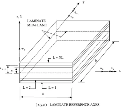
Fig 2.1 laminate geometries with positive set of lamina / laminate reference axes, displacement components.

2.2 Strain- Displacement relations:

By substitution of the displacement relations in Eq. (1) Into the strain displacement equations of the classical theory of elasticity, the following relations are obtained.

0

ε

* y k z *

yo

ε

z y zk yo

ε

y

ε

* x k z * xo

ε

z x zk xo

ε

x

ε

z

2

3 2

3



 

 

 

 

* x

φ

z xzo zε x

φ

xz

γ

* y

φ

z yzo zε y

φ

yz

γ

* xy k z * xyo

ε

z xy zk xyo

ε

xy

γ

2 2

3 2

  

 

 

(3)

* x 3θ * x φ , * y 3θ * y φ , * o 2u xzo ε , * o 2v yzo ε x wo x θ x φ , y wo y θ y φ x * o v y * o u * xyo ε , y * o v * yo ε , x * o u * xo ε x θ y θ * xy k , y θ * y k , x θ * x k ; x θ y θ xy k , y θ y k , x θ x k ; x vo y uo xyo ε ; y vo yo ε , x uo xo ε * y * x * y * x y x y x                                                            

2.3 Constitutive equations:

According to Hooke’s law stress is directly proportional to strain, for a laminate the stress strain relationship with respect to laminate reference axes is given by

                                                       xz yz xy y x 55 44 33 22 12 12 11 xz yz xy y x γ γ γ ε ε Q 0 0 0 0 0 Q 0 0 0 0 0 Q 0 0 0 0 0 Q Q 0 0 0 Q Q τ τ τ σ σ Eq. (3)

Where  = (x, y, x-y, yes, xz) t are the stresses



= (



x,



y, xy, yz, xz)t are the strains with respect to the axes

Qij’s are the plane stress reduced elastic coefficients in the plate axes that vary through the plate thickness are

given by.                               2 44 2 55 55 44 55 45 2 55 2 44 44 4 4 66 2 2 66 12 22 11 33 3 66 22 12 3 66 12 11 23 4 22 2 2 66 12 4 11 22 3 66 22 12 3 66 12 11 13 4 4 12 2 2 66 22 11 12 4 22 2 2 66 12 4 11 11 sin Q cos Q Q sin cos ) Q Q ( Q sin Q cos Q Q ) cos (sin Q cos sin ) Q 2 Q 2 Q Q ( Q cos sin ) Q 2 Q Q ( cos sin ) Q 2 Q Q ( Q cos Q cos sin ) Q 2 Q ( 2 sin Q Q cos sin ) Q 2 Q Q ( cos sin ) Q 2 Q Q ( Q ) cos (sin Q cos sin ) Q 4 Q Q ( Q sin Q cos sin ) Q 2 Q ( 2 cos Q Q                                     

.

Eq. (4)

Where 23 44 12 55 66 21 12 2 22 22 12 12 21 12 1 11 Q Q Q υ υ 1 E Q Q * υ Q υ υ 1 E Q g g        

2.4 Equations of Motion:

Hamilton Principle can be written in analytical form as follows:

(4)

Where U is the total Potential strain energy due to deformations, V is the potential of the external loads, K the kinetic energy and U+V=π is the total potential energy. Substituting the appropriate energy expressions the final expression can be written as

0 ] [ 2 / ) ( ( 2 2 2 0 2 / 2 / 2 / 2 / 0         



  

 



  dAdzdt w v u wdA p dAdz o o o A t h h A z zx zx yz yz xy xy y y x x h h A t                 Eq (6) Where ρ is the mass density of the material and Pz the transverse load applied at the top surface of the plate.

Using Eqns. (1), (2) in Eq. (6) and integrating the resulting expression by parts and collecting the coefficients of

δuo, δvo, δwo, δƟx, δƟy, δuo*, δvo*, δƟx*, δƟy* the following equations are obtained:

* x 4 * 0 3 x 2 0 1 xy x

0

I

u

I

(

θ

)

I

u

I

θ

y

N

x

N

:

δ

u























* y 4 * 0 3 y 2 0 1 xy y

0

I

v

I

(

θ

)

I

v

I

θ

x

N

y

N

:

δ

v























0 1 y x

0

q

I

w

y

Q

x

Q

:

δ

w













* x 5 * 0 4 x 3 0 2 x xy x

x

Q

I

u

I

(

θ

)

I

u

I

θ

y

M

x

M

:

δθ

























* y 5 * 0 4 y 3 0 2 y xy y

y

Q

I

v

I

(

θ

)

I

v

I

θ

x

M

y

M

:

δθ

























* x 6 * 0 5 x 4 0 3 x * xy * x *

0

2S

I

u

I

(

θ

)

I

u

I

θ

y

N

x

N

:

δ

u

























* y 6 * 0 5 y 4 0 3 y * xy * y *

0

2S

I

v

I

(

θ

)

I

v

I

θ

x

N

y

N

:

δ

v

























* x 7 * 0 6 x 5 0 4 * x * xy * x *

x

3 Q

I

u

I

(

θ

)

I

u

I

θ

y

M

x

M

:

δθ

























* y 7 * 0 6 y 5 0 4 * y * xy * y *

y

3 Q

I

v

I

(

θ

)

I

v

I

θ

x

M

y

M

:

δθ

























Eq. (7)

The boundary conditions are given below. At edge x = 0 and x = a

v0 = 0, wo = 0, y = 0, z = 0, Mx = 0, v0* = 0, w0* = 0,

y* = 0, z* = 0, Mx* = 0, Nx = 0, Nx* = 0. Eq. (8)

At edges y = 0 and y = b

u0= 0, wo = 0, x = 0, z = 0, My = 0, u0* = 0, w0* = 0,

x* = 0, z* = 0, My* = 0, NY = 0, Ny* = 0. Eq. (9)

Where the stress resultants are defined by

 

1 |

z

dz

τ

σ

N

|

N

|

N

|

N

2 xy y x 2 h 2 h n 1 L * xy xy * y y * x x















































 

(5)



z

|

z



dz

τ

σ

M

|

M

|

M

|

M

3 xy y x 2 h 2 h n 1 L * xy xy * y y * x x















































 

Eq.(11) And the transverse force resultants and the inertias are given by:



1 |

z

|

z



dz

τ

Q

|

S

|

S

|

Q

|

Q

2 yz xz 2 h 2 h n 1 L * y * x y x y x



































 

Eq.(12) The resultants in Eq. (10), (11) & (12) can be related to the total strains in Eq. (2) By the following matrix:



























































* * s * 0 0 s b t * * *

φ

K

ε

D

|

0 |

0

0 |

D

|

B

0 |

B

|

A

Q

M

N

.

Eq. (14)

Where the matrices [A],[B], [Db] & [Ds] are the matrices of plates stiff nesses whose elements can be calculated

by using Eq.(3) And (4)

2.5 Navier method:

Navier method can be used to solve the governing equations of various laminated plates for which all four edges of laminate are simply supported.

For cross-ply laminates with edges y=0 and y=b simply supported and the other two edges x=0 and x=a simply supported. Assume the following representation of the displacement:

y

x

U

t

y

x

u

mn n m





sin

cos

)

,

(

1 1

0



   



y

x

V

t

y

x

v

_mn n m





cos

sin

)

,

(

1 1

0



   



y

x

W

t

y

x

w

_mn n m





sin

)

,

(

1 1

0



   



Eq. .(15)

y

x

V

t

y

x

v

mn n m

o

(

,

)

sin



cos



* 1 1 *



   



y

x

X

t

y

x

_mn n m

x







(

,

)

*

cos

sin

1 1 *



   



y

x

Y

t

y

x

mn n m

y







(

,

)

sin

cos

1 1



   



y

x

U

t

y

x

u

mn n m





sin

cos

)

,

(

* 1 1 *

0





 



(6)

y

x

Y

t

y

x

mn

n m

y







(

,

)

*

sin

cos

1 1 *





 



The Mechanical load is expanded in double Fourier sine series as:

y

x

Q

y

x

q

_mn

n m





sin

)

,

(

1





 



Eq

.

(16)

Where  =

a

m



The displacements in the mid plane will be defined to satisfy the boundary conditions. These displacements will be substituted in governing equations to obtain the equations in terms of A, B, Db and Ds matrix. The obtained equations

will be solved to find the behavior of the laminated composite

plates.

_























































₄ 2 2₂ 2₂ 2₂

3

,

100 qa

h

qa

h

qa

h

qa

E

h

w



x



x



y



y



xy



xy

The transverse displacement and stresses are evaluated at the following specified points as given below: Transverse displacement (w): (a/2, b/2, 0).

In-plane normal stress (σx): (a/2, b/2, ±h/2). In-plane normal stress (σy): (a/2, b/2, ±h/2). In-plane shear stress (τxy): (0, 0, ±h/2)

4. Results and Discussion

In this section, various numerical examples solved are presented for establishing the accuracy of the HSDT for the bending analysis of laminated composite plates

The material properties of the plate adopted here for the laminated composite plate as follows

Graphite-epoxy:

E1/E2=25, G12=G13=0. 5E2, G23=0. 2E2, ν12=ν23=ν31=0. 25

Table 3.1 compares the normalized central deflection of [0/90] and [0/90]10 laminated square plate with analyses

based on the third-order and Higher-order shear deformation plate. All numerical results are presented in the Tables 3.1 in non- dimensonalized form as w =100w ×E2h3/qoa4

Table:3.1 Parametric study of Deflections for [0,90], [0.90]10 graphite-epoxy square under sinusoidal loading

BC No of layers a/h TSDT Present % of error

SS

2 5 1.667 1.6914 1.40%

10 1.216 1.216 0%

10 5 1.129 1.116 1.50%

10 0.616 0.585 4.90%

Table:3.2 Material properties (GPa)

Materials E1 E2 E3 G12 G12 ν12 ν23 ν31

Boron/Epoxy 206.9 20.7 20.7 5.2 5.2 0.3 0.3 0.3

Carbon/Epoxy 206.9 5.2 5.2 5.2 2.6 0.25 0.25 0.25

Glass/Epoxy 53.8 17.9 17.9 8.9 8.9 0.25 0.25 0.25

Table 3.2 shows different material properties used for each lamina of the laminated composites to study the effect of side to thickness ratio, aspect ratio and stacking sequence on deflection.From the table 3.1 it is observed that the maximum % of error between TSDT and present HSDT is 4.90% for 10 layers.

(7)

Figs show the outcome result from deflection, normal stresses and shear stresses from different side to thickness ratios, aspect ratios and various layers and several fiber orientations. It was noted that different side to thickness ratio affected the deflection. Figures show the outcome result from deflection, normal stress and shear stress from different side to thickness ratios in various layers and several fiber orientations. Minimum number of layers against maximum advantage is the most important factors in optimization, design and manufacturing of composite materials to decrease the deflection and the existing stresses. As it is illustrated, increasing the number of layers does not have much of an effect in fiber orientations 15/-15, 45/-45 and 60/-60, however in fiber orientation 90, increasing the layers, to some extend, concludes to a higher deflection, although it still has obvious difference against other orientations, which is because of the increasing stiffness in the D matrix

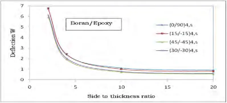
Fig 3.1contain plots of deflection versus side to thickness ratio (a/h) of various angle ply laminates subjected to uniformly or sinusoid ally distributed transverse load. The effect of transverse shear deformations negligible for all valves of (a/h) greater than 10.For valves of (a/h) less than 10, the effect is quite significant. The deflection and normal stress are given at center of plate and transverse shear at the middle of the sides. It is clear that the deflection increases as the side-to thickness ratio decreases the difference increases for deflection w. The Boron having higher deflection at [45,-45]8 ad having low deflection at [0,90]8 orientations. While

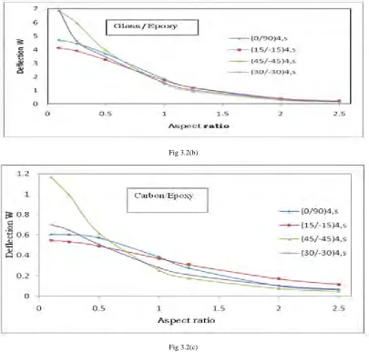
carbon having lower deflections and glass having high deflections when compared with Boron and carbon Fig 3.2 shows the effect of bending-stretching coupling and plate aspect ratio on the transverse deflections (W), normal stresses and shear stresses (σx, σy andτxy). The deflections decrease as the aspect ratio (a/b) increases. The difference increases as the aspect ratio increases while it may be unchanged with the increase of side-to-thickness ratio. It is observed that, the non-dimensional deflection is maximum for a/b =0.1 .This is due to the fact that, as the young’s modulus of the material increases. The effect of coupling is to decrease the deflections and stresses. The coupling coefficients increase in magnitude (hence the effect of coupling increases) with the increase of the aspect ratio for deflections (W) and decrease of modulus ratio for stresses and also, the effect of coupling on deflections is quite significant for aspect ratio less than 1and is negligible for all values of a/b greater than 2.5. The effect of coupling is to decrease the stresses with the increase in aspect ratios.This is because the plate area increases as the aspect ratio increases and hence, the applied load per unit area decreases. The effect of transverse shear deformation is to decrease the deflections and increase stresses with the increase in the modulus ratio and side-to-thickness ratio

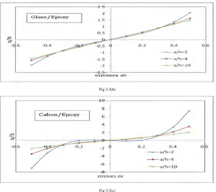
Fig 3.3 Computed centroidal deflection, axial in-plane stress at the center of the top surface, and through-the-thickness variation of the deflection, the axial stress at points on the vertical line passing through the centroid, and the transverse shear stress at points on the vertical line passing through the point (0, a/2, 0) of a simply supported square the in-plane longitudinal and normal stresses, (σx) and (σy) , are compressive throughout the plate up to z =- 0.55 and then they become tensile. The maximum compressive stresses occur at a point on the bottom surface and the maximum tensile stresses occur, of course, at a point on the top surface of the plate.

However, the tensile and compressive values of the longitudinal tangential stress, τxy, are maximum at a point on the bottom and top surfaces of the plate, respectively. It is clear that the minimum value of zero for all. In-plane stresses σx, σy and τxy occurs at z = 0.5 and this is irrespective of the aspect and side-to-thickness ratios. This is due to the fact that, the plate area increases as the side to thickness ratio increases and hence, the applied load per unit area decreases as the young’s modulus of the material increases.

(8)

Fig:3.1.(b)

Fig:3.1.(c)

Fig 3.1: Deflection vs. various sides to thickness ratio, fiber orientations and different material properties

(9)

Fig 3.2(b)

Fig 3.2(c)

Fig 3.2: Deflection vs for various Aspect ratio, fiber orientations and different material properties

(10)

Fig 3.3(b)

Fig 3.3(c)

Fig 3.3: z/h vs stresses (σx) for various fiber orientations and material properties

(11)

Fig 3.5: z/h vs stress (σx) shear stresses (τyz) for fiber orientations and material properties

4. Conclusions

In this paper a analytical method is developed to find the bending characteristics of laminated composite plates using higher order theory. A unified general formulation of all higher order theories has been presented for composite based on a polynomial expansion of displacement in the thickness coordinate. The results may be important to the designer in the field of laminated composite construction .It was noted that different side to thickness ratio affected the deflection. The deflection decreases as side to thickness ratio increases. The decrease of the deflection is uniform with the increase of side to thickness ratio. It is observed that, the deflections are larger for smaller modulus ratio and aspect ratios. Comparisons of the results with those available in the literature and results of finite element method show good agreements with small acceptable deviation. It has been shown that the value in HSDT is higher than that in TSDT. Hence, the rapid changes of deflection at the edges are more significant in HSDT. Since HSDT predicts the deflection components more accurate than TSDT. This is an important result that should be considered in the design of laminated plates

5. References

[1] Leissa A.W., Vibration of plates, NASA, SP-160, (1969).

[2] Reissner E., The effect of transverse shear deformation on the bending of elastic plates, J.Appl. Mech., (1945), 12, p. 69-77. [3] Reissner E., On the theory of bending of elastic plates, J. Math. Phys., (1944), 23, p. 184-191.

[4] Midlin R.D., Influence of rotatory inertia and shear on flexural motions of isotropic,elastic plates, J. Appl. Mech., (1951), 18, p. 31-38.

[5] Whitney J.M., Pagano N.J., Shear deformation in heterogeneous anisotropic plates, J.Appl. Mech., (1970), 37, p. 1031-1036. [6] Liew K.M., Xiang Y., Kitipornchai S., Transverse vibration of thick rectangular plates-I. Comprehensive sets of boundary

conditions, Comp. Struct. (1993), 49, p. 1-29.

[7] Whitney J.M., Sun C.T., A higher order theory for extensional motion of laminated composites, J. Sound Vibr. (1973), 30, p. 85-97.

[8] Whitney, J.M., Sun C.T., A refined theory for laminated, anisotropic, cylindrical shells, J.Appl. Mech. (1974), 41, p. 471-6. [9] Gautham B.P., Ganesan N., Free vibration analysis of thick spherical shells, Comp.Struct. (1992), 45(2), 307-13.

[10] Hildebrand FB, Reissner E, Thomas GB. Note on the foundations of the theory of small displacements of orthotropic shells. NACA TN-1833, (1949).

[11] Nelson RB, Lorch DR. A refined theory for laminated orthotropic plates. ASME J Appl Mech (1974);41:177–83.

[12] Librescu L. Elastostatics and kinematics of anisotropic and heterogeneous shell type structures. The Netherlands: Noordhoff;(1975).

[13] Lo KH, Christensen RM, Wu EM. A higher order theory of plate deformation, Part 1: Homogeneous plates. ASME J Appl Mech (1977)a;44(4):663–8.

(12)

[15] Levinson M. An accurate simple theory of the statics and dynamics of elastic plates. Mech Res Commun (1980);7:343. [16] Murthy MVV. An improved transverse shear deformation theory for laminated anisotropic plates. NASA Technical

Paper-1903,(1981).

[17] Whitney JM, Pagano NJ. Shear deformation in heterogeneous anisotropic plates. ASME J Appl Mech 1970;37(4):1031–6. [18] Reddy JN. A simple higher order theory for laminated composite plates. ASME J Appl Mech (1984);51:745–52

[19] Pagano NJ. Exact solutions for rectangular bidirectional composites and sandwich plates. J Compos Mater 1970;4(1):20–34. [20] Reddy JN. Energy and variational methods in applied mechanics. New York: Wiley; (1984).