https://doi.org/10.5194/cp-15-957-2019
© Author(s) 2019. This work is distributed under the Creative Commons Attribution 4.0 License.
Ocean-driven millennial-scale variability of the Eurasian ice
sheet during the last glacial period simulated
with a hybrid ice-sheet–shelf model
Jorge Alvarez-Solas1,2, Rubén Banderas1,2, Alexander Robinson1,2, and Marisa Montoya1,2
1Departamento de Física de la Tierra y Astrofísica, Facultad de Ciencias Físicas,
Universidad Complutense de Madrid (UCM), Madrid, Spain
2Instituto de Geociencias (UCM-CSIC), Madrid, Spain
Correspondence:Jorge Alvarez-Solas ([email protected])
Received: 20 July 2018 – Discussion started: 9 October 2018
Revised: 30 April 2019 – Accepted: 6 May 2019 – Published: 4 June 2019
Abstract.The last glacial period (LGP; ca. 110–10 kyr BP) was marked by the existence of two types of abrupt cli-matic changes, Dansgaard–Oeschger (DO) and Heinrich (H) events. Although the mechanisms behind these are not fully understood, it is generally accepted that the presence of ice sheets played an important role in their occurrence. While an important effort has been made to investigate the dynam-ics and evolution of the Laurentide ice sheet (LIS) during this period, the Eurasian ice sheet (EIS) has not received much attention, in particular from a modeling perspective. However, meltwater discharge from this and other ice sheets surrounding the Nordic seas is often implied as a potential cause of ocean instabilities that lead to glacial abrupt climate changes. Thus, a better comprehension of the evolution of the EIS during the LGP is important to understand its role in glacial abrupt climate changes. Here we investigate the re-sponse of the EIS to millennial-scale climate variability dur-ing the LGP. We use a hybrid, three-dimensional, thermo-mechanical ice-sheet model that includes ice shelves and ice streams. The model is forced off-line via a novel perturbative approach that, as opposed to conventional methods, clearly differentiates between the spatial patterns of millennial-scale and orbital-scale climate variability. Thus, it provides a more realistic treatment of the forcing at millennial timescales. The effect of both atmospheric and oceanic variations are included. Our results show that the EIS responds with en-hanced ice discharge in phase with interstadial warming in the North Atlantic when forced with surface ocean temper-atures. Conversely, when subsurface ocean temperatures are used, enhanced ice discharge occurs both during stadials and
at the beginning of the interstadials. Separating the atmo-spheric and oceanic effects demonstrates the major role of the ocean in controlling the dynamics of the EIS on millen-nial timescales. While the atmospheric forcing alone is only able to produce modest iceberg discharges, warming of the ocean leads to higher rates of iceberg discharges as a result of relatively strong basal melting at the margins of the ice sheet. Our results clearly show the capability of the EIS to re-act to glacial abrupt climate changes, and highlight the need for stronger constraints on the ice sheet’s glacial dynamics and climate–ocean interactions.
1 Introduction
Preceding these, and concomitant with the culmination of the prolonged stadials, H-events are registered in North Atlantic marine sediments as layers of remarkably high concentra-tions of ice-rafted debris (IRD) (Heinrich, 1988) as a result of massive iceberg discharges from the Laurentide ice sheet (LIS) (Hemming, 2004).
While significant effort has been invested in understand-ing the role of the LIS in glacial abrupt climate changes, the dynamics of the Eurasian ice sheet (EIS) during the LGP has received comparatively less attention from a modeling per-spective. However, improving our understanding of the evo-lution of the EIS and its response to past climate changes is important for a number of reasons. First, constraining fresh-water inputs into the North Atlantic Ocean is crucial for a better understanding of the driving mechanisms of glacial abrupt climate changes (Rasmussen and Thomsen, 2013), as meltwater discharge from the ice sheets surrounding the Nordic seas is often implied as a cause of ocean instabil-ities. Precursor events could possibly have originated from the European and Icelandic ice sheets (Grousset et al., 2000; Scourse et al., 2000). Meltwater peaks in the Norwegian Sea as well as in the southern border of the EIS during Ma-rine Isotopic Stage 3 (MIS 3; ca. 60–25 kyr BP) have been associated with H-events and millennial-scale climate vari-ability (Lekens et al., 2006; Toucanne et al., 2015). From a broader perspective, the EIS, consisting of the Fennoscan-dian, the British Isles and the Barents–Kara ice sheets (FIS, BIIS and BKIS, respectively) contained a large marine-based sector at its maximum extension (Hughes et al., 2016) that was exposed to oceanic variations. The BKIS, in particular, was predominantly marine-based for much of the LGP. For this reason, and because it had a size similar to the West Antarctic ice sheet (WAIS) during the Last Glacial Maxi-mum (LGM) (Anderson et al., 2002; Bentley et al., 2014; Denton and Hughes, 2002; Evans et al., 2006; Hillenbrand et al., 2012; Svendsen et al., 2004; Whitehouse et al., 2012), it is sometimes considered as a geological analog of the cur-rent WAIS (e.g., Gudlaugsson et al., 2013). However, while the WAIS endured the deglaciation, the BKIS completely disappeared (Andreassen and Winsborrow, 2009). Mecha-nisms contributing to the deglaciation of the BKIS include ice stream surging (Andreassen and Winsborrow, 2009), sub-glacial meltwater (Esteves et al., 2017) and subsurface melt-ing via ocean warmmelt-ing (Ivanovic et al., 2018; Rasmussen and Thomsen, 2004). An improved understanding of these mech-anisms would provide important insights into the future evo-lution of the WAIS (Gudlaugsson et al., 2013, 2017).
Reconstructing the evolution of glacial ice sheets prior to the LGM has been difficult, in part because, in reach-ing their maximum extent, ice sheets eroded and removed nearly all older deposits. This has particularly hampered the reconstruction of the EIS response to past glacial abrupt cli-mate changes. Nevertheless, the available paleodata indicate that during MIS 3 the EIS was highly dynamic, with its ad-vance and retreat closely linked to stadials and
interstadi-als (Toucanne et al., 2015). In this line, records from Nor-way (Mangerud et al., 2003; Mangerud et al., 2010; Olsen et al., 2002), Finland (Helmens and Engels, 2010) and Swe-den (Wohlfarth, 2010) indicate rapid and rhythmic ice-sheet variations in Scandinavia, with advances and retreats during stadials and interstadials, respectively. Recent records also indicate enhanced meltwater discharges during interstadials from the Svalbard–Barents Sea ice sheet and probably also from the Scandinavian ice sheet (Rasmussen and Thomsen, 2013). The resolution and quality of geophysical data across marine sectors have improved considerably over the past decade (Hughes et al., 2016, and references therein). These data confirm substantial variations of the EIS extent, with the largest uncertainties in marine sectors of the ice sheets; as a consequence, trying to estimate its limits prior to 32 kyr BP was not attempted by Hughes et al. (2016). Strong variations in the deposition of IRD suggest high co-variability of BIIS-sourced calving events with changes in ocean sea surface temperature (Hall et al., 2011; Scourse et al., 2009) and vari-ations in EIS ice streams (Becker et al., 2017). North Atlantic marine sediment records register widespread variations of IRD input throughout the LGP, indicating variations of ice-berg rafting from virtually all surrounding ice sheets. Sources and timing differ among different sites. A dominant period-icity equal to that of DO-events was identified in sediment records from the Irminger Sea, with the largest IRD peaks at the end of stadials originating in the Iceland and Greenland ice sheets (von Kreveld et al., 2000). Strong millennial-scale iceberg rafting variability of the BIIS has been documented in sediment records from the North Sea (Hall et al., 2011; Peck et al., 2007; Scourse et al., 2009), but enhanced IRD seems to occur both during interstadials and stadials. For the FIS, IRD records in the Norwegian Sea show the characteris-tic DO periodicity, with IRD discharge occurring just before stadial–interstadial transitions (Lekens et al., 2006). More recently, however, an increase in IRDs from Fennoscandia during interstadials has been reported (Dokken et al., 2013; Becker et al., 2017). Nevertheless, correlating IRD occur-rence with temperature changes registered in Greenland re-mains difficult because it requires an extremely well-dated chronology to assess the phasing between ocean sediments and ice cores.
in-troducing a simple representation of the subglacial hydro-logical system, focusing on its role in the temporal evolu-tion of the EIS. Recently, an ice-sheet model constrained by data has been used to simulate the EIS evolution through-out part of the LGP, from 37 to 19 kyr BP (Patton et al., 2016). This study was subsequently extended throughout the last deglaciation until 8 kyr BP (Patton et al., 2017). The model targets the most probable EIS distribution at different time slices and reproduces substantial ice-volume variations. However, all of these models suffer from limitations, such as the use of the shallow-ice approximation (SIA) and its as-sociated lack of an explicit treatment of the oceanic forcing. Marshall and Koutnik (2006) investigated the production of icebergs from all of the North American ice sheets with a pa-rameterized calving model. They found different behaviors on millennial timescales depending on the local glaciolog-ical and climatic characteristic, with increased iceberg pro-duction during both stadials (e.g., from Iceland) and intersta-dials (e.g., from Barents Sea). Nonetheless, submarine melt-ing at the groundmelt-ing line has not been explicitly considered until now and its impacts on millennial-scale variability have not been investigated up until this point from a modeling per-spective. Notable exceptions are the recent studies by Petrini et al. (2018) and Åkesson et al. (2018). The latter used a high-resolution ice-sheet model with an accurate representation of the grounding-line dynamics to study the deglaciation of the marine-based southwestern section of the Scandinavian ice sheet; however, the model domain was limited to a very small region within southwest Norway.
Here, we investigate the response of the EIS to millennial-scale climate variability during MIS 3 using a three-dimensional ice-sheet model. To this end, a novel off-line approach is used that provides a better representation of millennial-scale climate variability (Banderas et al., 2018). In addition, for the first time, both the atmospheric and oceanic effects of millennial-scale climate variability associated with glacial abrupt climate changes are considered. This facilitates the quantification of the relative contribution of surface (ab-lation) and dynamic processes related to ice–ocean interac-tions.
The paper is organized as follows: in Sect. 2 the ice-sheet model, the forcing method and the experimental setup are described. In Sect. 3 the response of the EIS to the imposed forcing is shown, the focus being the evolution of its ice vol-ume, its impact on sea level and the mechanisms behind melt-water and ice discharge. In Sect. 4 the implications of our study for glacial and future climate changes are discussed. Finally, the main conclusions are summarized in Sect. 5.
2 Model and experimental setup
2.1 Model
The model used in this study is the GRISLI-UCM ice-sheet model, an extension of the original GRISLI model
devel-oped by Ritz et al. (2001). GRISLI-UCM is a hybrid three-dimensional thermomechanical ice-sheet model. Inland ice flows through deformation under the shallow-ice approxi-mation (SIA, Hutter, 1983). The underlying assumption is that the flow is dominated by bed-parallel vertical shear for grounded ice (i.e., shear or deformational flow).
A nonlinear viscous flow law (the Glen flow law) is used with an exponentn=3. Viscosity depends on temperature through an Arrhenius law. A traditional enhancement fac-tor,Ef, that decreases viscosity and accelerates inland flow is
used in most ice-sheet models as a tuning parameter, in order to improve the agreement between modeled and measured ice thicknesses; hereEf=3. Further details can be found in
Ritz et al. (2001). Thermomechanical coupling is extended to the ice shelves and ice streams. Ice viscosity, dependent on the temperature field, is integrated over the thickness, as in Peyaud et al. (2007). Ice shelves and ice streams are described following the shallow-shelf approximation (SSA, MacAyeal, 1989). In such fast flow areas bed-parallel shear is no longer dominant; instead, longitudinal and lateral stresses become important in such a way that the horizontal velocity is independent of depth (plug flow). Both approximations are valid when the spatial scale is much smaller in the vertical di-rection than in the horizontal didi-rection, as is the case in large-scale ice-sheet modeling. Ice streams (areas of fast flow, typ-ically faster than 102m a−1) are considered to be dragging ice shelves, allowing for basal movement of the ice (Bueler and Brown, 2009). Basal stress under ice streams (τb) is
pro-portional to the ice velocityuband to the effective pressure
of iceNeff representing the balance between ice and water
pressure:
τb= −fub, (1)
where
f =cfNeff. (2)
Herecfis an adjustable basal friction coefficient related to the
bedrock topography that accounts for the basal type of mate-rial. The effects of varying this proportionality factor on the simulated ice streams are discussed in Álvarez-Solas et al. (2011b). In this study,cf values of 20 and 2×10⁻⁵a m−1
were used for ice streams over bedrock and sediments, re-spectively, accounting for the lower basal friction in the latter case. For comparison, absolute values up to 7×10⁻⁴a m−1 were inferred by Morlighem et al. (2013) in Antarctica, with a very heterogeneous distribution; low coefficient val-ues were inferred in areas of fast motion dominated by slid-ing.Neffis calculated as
Neff=ρgH−ρwg(h−b), (3)
where ρ and ρw are the densities of ice and water, H is
not subject to confining pressure, calculated within the basal hydrology scheme implemented by Peyaud (2006). Thus, the first term on the right hand side represents the pressure due to the ice load, and the second term represents the subglacial water pressure. At the base of the ice shelves, friction (and thus basal drag) is set to zero. The locations of the ice streams are determined by the presence of basal water within areas where the sediment layer is saturated. The criterion to acti-vate SSA inland relies on the presence of water above 1 m in regions of soft sediments (Laske, 1997) and above 400 m in the absence of such sediments. Setting these thresholds ensures that ice streams are activated in regions that are ro-bustly temperate. The presence of water at the base of the ice sheet implies that it is not frozen to the bedrock, i.e., sliding is physically possible. More water at the base further facilitates sliding by reducing the effective pressure, and sediments also facilitate sliding because they are deformable. The criteria of 1 m water thickness over sediments reduces noise in the SSA activation. The 400 m criterion over hard bedrock is a tunable parameter, which also allows for a more numerically robust calculation of velocities within the SSA. The grounding-line position dynamically evolves following the flotation criterion after the mass conservation equation is solved.
Calving takes place at the ice-shelf front when two con-ditions are met. First, the ice-shelf thickness must fall below a thresholdHcalv. This is a semiempirical parameter
reflect-ing the fact that this is the typical thickness of ice-shelf fronts currently observed in Antarctica (Griggs and Bamber, 2011). Second, the upstream advection must fail to maintain the ice thickness above this threshold following a semi-Lagrangian approach (Peyaud et al., 2007) to account for the fact that ice-flux divergence fosters the formation of crevasses (Lev-ermann et al., 2012). This method is standard in the GRISLI model. It was introduced after recognizing that a systematic cutoff of ice shelves below a given threshold led to a realis-tic simulation of the present-day ice shelves in Antarcrealis-tica, as is the case in many models, but prevents any develop-ment of new ice shelves (Peyaud, 2006; Peyaud et al., 2007). When focusing on past climates, ice sheets should be able to evolve in response to climate changes, and in particular to allow the advance of ice shelves in cold climates. To this end, before calving ice in a certain point, we test whether advection allows for the growth of ice at the front, and there-fore the ice-shelf advance. Hcalv was set to 150 m, in the
standard setup. To assess the sensitivity of the ice dynamics to the value of the thickness threshold Hcalv (below which
the ice is calved) we performed a new ensemble exploring a wide value range of this parameter’s values, from 10 to 800 m (Fig. S4 in the Supplement). Values of this threshold above 400 m produce a drastic disintegration of the Barents–Kara complex due to its relative shallow bed. The overall effect of this sensitivity test around the preferred value is to mod-ulate the amplitude of the response to the oceanic perturba-tions. Thus, GRISLI-UCM explicitly calculates grounding-line migration in addition to ice-stream and ice-shelf
ve-locities. This allows the model to properly represent both grounded and floating ice. Note that there is no ambiguity in the model between calving and basal melt, which are two distinct processes in the model. Calving is the result of the threshold criterion described above; thus, the calving rate at a given time is given by the amount of ice lost to the ocean through this process by unit of time, converted to mass-water equivalent. Basal melt is dependent on the applied ocean temperature anomaly. GRISLI-UCM uses finite differences on a staggered Cartesian grid at a 40 km resolution, corre-sponding to 224×208 grid points for the Northern Hemi-sphere domain, including the EIS, with 21 vertical levels. By default, initial topographic conditions are provided by sur-face and bedrock elevations built from the ETOPO1 dataset (Amante and Eakins, 2009) and ice thickness (Bamber et al., 2001). Note there are more recent datasets for Greenland topographic features (e.g., Bamber et al., 2013; Morlighem et al., 2014; Morlighem et al., 2017). However, as Greenland is not the focus of our study, this does not affect our results. The glacial isostatic adjustment (GIA) is described by the elastic lithosphere–relaxed asthenosphere method (Le Meur and Huybrechts, 1996), for which the viscous asthenosphere responds to the ice load with a characteristic relaxation time for the lithosphere of 3000 years. For the sake of simplicity, in this study the isostatic adjustment is assumed to be only due to local ice mass variations, as other such research has assumed in the past (e.g., Greve and Blatter, 2009; Helsen et al., 2013; Huybrechts, 2002; Langebroek and Nisancioglu, 2016; Stone et al., 2010). The surface mass balance (SMB) is given by the sum of accumulation and ablation, both of which are calculated from monthly surface air temperatures (SATs) and monthly total precipitation. Accumulation is cal-culated by assuming that the fraction of solid precipitation is proportional to the fraction of the year with mean daily tem-perature below 2◦C. The daily temperature is computed from monthly SATs assuming that the annual temperature cycle follows a cosine function. Ablation is calculated using the positive-degree-day (PDD) method (Reeh, 1989). Its main parameters are the standard deviation of daily temperature, σ, and the conversion factors from PDDs to melt for snow and ice, fPDDsnow and fPDDice. Here, σ=5 K, fPDDsnow= 0.003 m.w.e. PDD−1 and fPDDsnow=0.008 m.w.e. PDD
−1.
fPDDice =0.008 m.w.e. PDD
−1. Refreezing is considered,
with a value of Csi=60 % (see Sect. 2 in the
GRISLI-UCM accounts for changes in elevation at each time step con-sidering a linear atmospheric vertical profile for temperature with different lapse rates in summer and in the annual mean (0.0065 and 0.0080 K m−1, respectively) to account for the smaller summer atmospheric vertical stability.
Basal melting for grounded ice depends on pressure and water content at the base of the ice sheet (Ritz et al., 2001) as well as on the geothermal heat flux, which is prescribed from the reconstruction by Shapiro and Ritzwoller (2004). Basal melting for floating ice is computed using a linear tempera-ture anomaly with respect to the freezing point. The details of the implementation of the boundary conditions (SMB and oceanic basal melting) in this particular study are given be-low (Sect. 2.2). Finally, ice fbe-low was calculated with a 1-year time step, whereas thermodynamics and boundary conditions (including PDD) were updated every 5 years. The model parameters and the range of their values explored here are shown in Table 1.
2.2 Off-line forcing method
SMB and oceanic basal melting are obtained through a time-varying synthetic climatology built with a novel method that is found to provide a more realistic off-line forcing for ice-sheet models than classical off-line methods (Banderas et al., 2018). The method follows a perturbative approach in the sense that the forcing combines the present-day climatol-ogy, obtained from observational data, and simulated anoma-lies. However, in contrast to usual off-line forcing methods, orbital- and millennial-scale variabilities are not lumped in a sole anomaly pattern but differentiated. Thus, the method combines present-day observations, simulated LGM anoma-lies relative to present, scaled by an orbital-timescale in-dex, and simulated stadial–interstadial anomalies, scaled by a millennial-timescale index:
Tatm(t)=T0atm+ 1−α?(t)
1Torbatm+β?(t)1Tmilatm (4) P(t)=P0α?(t)+ 1−α?(t)δPorb 1−β?(t)
+β?(t)δPmil . (5)
Here,Tatm(t) andP(t) are the SAT and precipitation fields at timet.T0atmandP0are the ERA-Interim present-day SAT
and precipitation climatologies (Dee et al., 2011).1Tatm orb =
Tlgmatm−Tpdatm andδPorb=Plgm/Ppd are the orbital
tempera-ture anomaly and precipitation ratio relative to the present day (not shown, see Banderas et al., 2018), respectively, ob-tained from previous equilibrium simulations for the prein-dustrial and LGM climates performed with the CLIMBER-3αmodel (Montoya and Levermann, 2008).1Tmilatm=Tisatm− Tstatm and δPmil=Pis/Pst are the millennial temperature
anomaly and precipitation ratio, respectively, for the inter-stadial relative to the inter-stadial state (Sect. 2.3). The key dif-ferences between these climate modes as simulated by Mon-toya and Levermann (2008) with the CLIMBER-3α model are that in the stadial, North Atlantic Deep Water (NADW)
formation is relatively weak and takes place south of Iceland. Accordingly the sea-ice front in the North Atlantic reaches 40◦N. In the interstadial state there is a northward shift and
intensification of NADW formation. Northward oceanic heat transport increases, and the North Atlantic and surround-ing areas warm relative to the stadial state, in particular the Nordic seas. Thus, the simulated interstadial state is charac-terized by a more vigorous NADW formation and Atlantic meridional overturning circulation (AMOC) along with re-duced sea ice in the Nordic seas, and a temperature increase of up to 10 K in the North Atlantic relative to the stadial state, with a maximum anomaly in the Nordic seas. Note that bold symbols indicate two-dimensional spatial fields. The stadial mode in our study is represented by a climate simulation of the LGM with CLIMBER-3α (Montoya and Levermann, 2008). The interstadial mode is taken from a re-cent glacial transient simulation performed with the same model under glacial climatic conditions, but with intensi-fied NADW formation (Banderas et al., 2015).α?andβ?are two indices that separately modulate the contribution of the orbital and millennial anomalies. Both were built based on two recent complementary temperature reconstructions over Greenland, one from the NGRIP ice-core record for the LGP (Kindler et al., 2014), and the other from several ice-core records for the Holocene (Vinther et al., 2009). Their combi-nation (hereafter, the KV reconstruction) results in a contin-uous temperature reconstruction for Greenland for the past 120 kyr (Banderas et al., 2018).α? is obtained after apply-ing a low-pass frequency filter (fc=1/18 ka−1) to the
orig-inal KV reconstruction based on a spectral decomposition; β? is obtained following a similar procedure but retaining the high-frequency signal. Both indices are tuned in such a way that the resulting synthetic temperature time series at the NGRIP site exactly matches the KV reconstruction (this dis-tinguishesα?andβ?from the rawαandβ indices previous to this tuning; Banderas et al., 2018).
The net basal melting rate for floating ice,B, is assumed to follow a linear relation:
B=κ(Tocn−Tf), (6)
whereTocn is the oceanic temperature close to the ground-ing line, Tf is the temperature at the ice base, which is
Table 1.Model parameters used in this study with their standard and explored values.
Variable/parameter Identifier name Standard value Explored range Units
Basal friction coefficient on sediments cf 2×10⁻⁵ – a m−1 Basal friction coefficient on bedrock cf 20×10−5 – a m−1 Standard deviation of daily temperature σ 5 (4–6) K
Snow conversion factor from PDDs to melt fPDDsnow 0.003 (0.0015–0.006) m w.e. PDD
−1 Ice conversion factor from PDDs to melt fPDDice 0.008 (0.004–0.016) m w.e. PDD
−1 Ice thickness threshold for calving Hcalv 150 (10–500) m
Oceanic sensitivity for ice-shelf melting κ 5 (0–10) m a−1K−1
difference can be linear (Beckmann and Goosse, 2003) or quadratic (Holland et al., 2008; Pollard and DeConto, 2012; DeConto and Pollard, 2016; Pattyn, 2017). The linear marine-shelf basal melting parameterization used in this study is the simplest case that allows for testing of the ice-sheet sensitivity to past oceanic temperature changes. Nevertheless, it accounts separately for basal melting below the ice shelves (away from the grounding line) and at the grounding line. The basal melting rate of the ice shelves (Bsh) is given by the grounding-line basal melt (Bgl) scaled
by a constant factor (γ):
Bsh=γ Bgl(t). (7)
In this study, γ is set to 0.1. Thus, we consider that the submarine melting rate for ice shelves is 10 times lower than that close to the grounding zone, which is in qualita-tive agreement with observations in some Greenland glaciers with floating tongues (Münchow et al., 2014; Wilson et al., 2017) as well as in Antarctic ice shelves (Rignot and Jacobs, 2002; Marsh et al., 2016). Note that this value is subject to uncertainty. Although we did not explore any other values different from γ=0.1, we did consider a range of κ val-ues between 1 and 10 m a−1K−1, which accounts for a wide range of oceanic sensitivities (see Sect. 2.3).
As in Peyaud et al. (2007), in regions with ocean depths above 750 m, an artificially large melting rate (20 m a−1 is
prescribed to avoid unrealistic growth of ice shelves beyond the continental-shelf break, where they would likely be sub-ject to high melt rates in reality because of high heat ex-changes with the ocean.
Following the approach described above, Tocn(t) is as-sumed to be given by an expression analogous to Eq. (4). Thus Eq. (6) can be rewritten as follows:
B=B0+κ 1−α?(t)1Torbocn+β?(t)1Tmilocn, (8)
whereB0=κ(T0ocn−Tf) represents the present-day oceanic
basal melting rate.
Finally, millennial-scale sea-level variations are prescribed according to the reconstruction by Grant et al. (2012, Sect. 2.3). The specific details of the experimental setup used are described below.
2.3 Experimental setup
In this study, we investigate the response of the EIS to millennial-scale climate variability during MIS 3. The start-ing point of our experiments is a control-run ice-sheet sim-ulation with constant boundary conditions for MIS 3 that provides a representative configuration of the EIS for that time period (Fig. 1). To this end,α? was set to its value at 40 ka BP, that is,α?=α40 K? = −0.1, andβ?=0 to preclude millennial-scale variations. Note, however, that these values are to a certain extent arbitrary; they are intended to provide a stable mean background state similar but not necessarily identical to background MIS 3 conditions. Thus,
T40 Katm=T0atm+ 1−α40 K? 1Torbatm (9) P40 K=P0
α40 K? + 1−α?40 KδPorb
(10)
B40 K=B0+κ 1−α40 K?
1Torbocn. (11)
Note that although Eq. (11) is formally correct and consis-tent with the scheme used, in contrast to the present-day SAT or precipitation the present-day rate of oceanic basal melt-ing cannot be determined. Thus, in practice we replace this equation by directly tuning the value ofB40 Kto obtain a
rea-sonable ice-sheet configuration at 40 kyr BP (Fig. 2) given the atmospheric forcing fields expressed by Eqs. (9)–(10). To this end, a constant basal melting rate of 0.1 m a−1is as-sumed. The ice sheet was forced with the resulting clima-tologies for 100 kyr previous to the start of the perturbations described below. This allows the vertical temperature profile within the ice sheet to be equilibrated with the climate. This procedure was found to facilitate the growth of European ice sheets within the reconstructed limits for 60 and 20 kyr BP (Svendsen et al., 2004; Kleman et al., 2013) (Fig. 2).
cli-Figure 1. Background climatic forcing for the control run (CTRL). MIS 3 (∼40 kyr BP) reference annual mean SAT(a)and summer mean SAT(b)in degrees Celsius and annual mean precipitation in meters per annum(c). Present-day contour lines with the land boundary delineated at a depth of−80 m are added for reference.
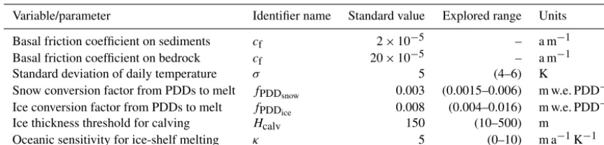
Figure 2. Resulting ice sheet of the MIS 3 control run (CTRL). Simulated ice thickness with contours plotted for every 500 m. The grounding-line position is shown using a black line, the 500 m depth contour is shown using a white line and velocities are shown us-ing the shaded colors (in kilometers per annum) after the spin-up was completed. This ice sheet represents the initial state previous to the application of perturbations. Bjørnøyrenna Basin, as referenced in the text, is shown using the black rectangle. The Barents–Kara, Scandinavian and British Islands regions are highlighted using blue, red and purple rectangles, respectively.
matic conditions. Thus,
Tatm(t)=T40 Katm+β?(t)1Tatmmil (12) P(t)=P40 K 1−β?(t)+β?(t)δPmil (13)
B(t)=B40 K. (14)
Second, an oceanic-only forced simulation (OCN) in which the atmospheric forcing is kept constant, while the oceanic basal melting is allowed to vary at millennial timescales around its background MIS 3 value:
Tatm(t)=T40 Katm (15)
P(t)=P40 K (16)
B(t)=B40 K+κ β?(t)1Tmilocn. (17)
The magnitude and sign of oceanic temperature anomalies 1Tocndepends on the depth at whichTocnis considered. In our simulations, a large part of the northeastern sector of the EIS is marine based with shallow bedrock depths between 500 m and less than 100 m in several locations further south. Therefore, it is unclear whether this marine ice sheet should be more susceptible to changes in the surface or the subsur-face of the ocean.
To investigate the effect of this uncertainty, we decided to perform two different simulations considering differ-ent depths: one corresponding to the surface (OCNsrf) and
the other considering deeper (subsurface) oceanic waters by averaging temperatures within the depth range of 400– 600 m (OCNsub). Therefore we hereafter distinguish between
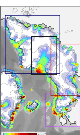
Figure 3.Millennial-scale components of the boundary forcing.(a)SAT anomalies (interstadial minus stadial) in degrees Celsius.(b) Sum-mer SAT anomalies (interstadial minus stadial) in degrees Celsius.(c)Precipitation ratio (interstadial to stadial).(d)Anomalies of SST and (e)subsurface ocean temperature (at a depth of 500 m) in degrees Celsius. Present-day contour lines with the land boundary delineated at a depth of−80 m are added for reference. Note that to force the ice-sheet model these fields are scaled to reproduce the NGRIP interstadial minus stadial temperature change.
Finally, a simulation “ALL” was carried out combining both the atmospheric and the oceanic forcings:
Tatm(t)=T40 Katm+β?(t)1Tmilatm (18) P(t)=P40 K 1−β?(t)+β?(t)δPmil (19)
B(t)=B40 K+κ β?(t)1Tmilocn. (20)
In all experimentsβ?(t) dictates the millennial-scale variabil-ity of the forcings (Fig. 4a). Because our simulated stadial– interstadial transition results from an intensification of the AMOC, positiveβ?values imply an increase inTatmrelative to its background MIS 3 value (e.g., Eq. 18; Figs. 3, 4). As a consequence, the atmosphere warms at interstadials relative to stadial periods, as reflected by the1Tmilatmmillennial-scale anomaly field (Fig. 3a, b). Note that refreezing is not allowed to occur in our current model setup. Ifκ β?1Tmilocn<−B40 K
(which would implyB(t)<0), we simply impose the value B(t)=0.
An ensemble of simulations for different values ofκhave been considered to evaluate the sensitivity of the EIS to the forcing. Finally, varying sea-level forcing is considered (Fig. 4b), both alone (SL) and in combination with the previ-ous forcings (ALL).
3 Results
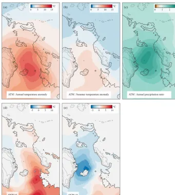
Table 2.Millennial-scale components used to force the ice-sheet model in the different experiments shown in this study.
Experiment name Millennial-scale forcing component
Atmosphere Surface ocean Subsurface ocean Sea level
CTRL · · · ·
SL · · · X
ATM X · · ·
OCNsrf · X · ·
OCNsub · · X ·
ALLsrf X X · X
ALLsub X · X X
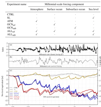
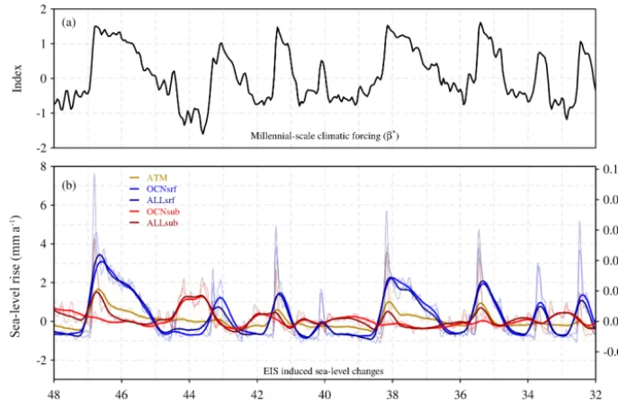
Figure 4.(a)Temporal component of the millennial-scale climatic forcing (β?index).(b)Millennial-scale sea-level forcing (Grant et al., 2012).(c)EIS sea-level equivalent (in meters) related to ice volume variations (in cubic meters) with respect to initial conditions for the CTRL run (black) and for the SL (gray), ATM (gold), OCNsrf(blue), OCNsub(red), ALLsrf(dark blue) and ALLsub(dark red) forcing experiments.
3.1 Ice volume evolution
Substantial differences are found in the response of the EIS to the forcing scenarios. Under constant forcing, the CTRL run shows negligible millennial-scale sea-level equivalent (SLE) variations, although a lower frequency SLE fluctuation is found as a result of internal ice-sheet variability (Fig. 4) through a thermomechanical feedback. This slow variabil-ity appears only in the southernmost parts of the Eurasian ice sheet where ablation exists. It is due to an interplay be-tween the available basal water favoring sliding and the EIS associated thinning due to an increase in velocities. As this phenomenon concerns only the ablative borders of the ice sheet and its frequency corresponds to more than 20 kyr, its governing dynamics is not detailed here. When the model is forced only by changes in sea level (SL run), a small response of approximately 0.5 m SLE is observed on millennial scales.
These changes appear not to be sufficient to cause a substan-tial migration of the grounding line, and thus do not affect ice velocities (not shown). In ATM, the atmospheric forcing alone causes a sequence of enhanced ablation episodes re-sulting in modest ice volume variations (up to 1.5 m SLE) during the most prominent stadial–interstadial transitions; this represents a change of approximately 7 % with respect to the initial ice-sheet volume. In contrast, the oceanic forc-ing in OCNsrf induces pronounced changes in the
dynam-ics of the EIS on millennial timescales (see below), with episodes of large volume reduction occurring during intersta-dials. The combination of sea level, atmospheric and oceanic forcings (ALLsrf) results in a very similar response of the EIS
to that obtained in OCNsrf(Fig. 4) as a consequence of the
larger effect of the oceanic forcing in OCNsrfwith respect to
Figure 5.MIS 3 period.(a)Temporal component of the millennial-scale climatic forcing (β?index), and(b)EIS changes (in millimeters per annum and Sv) related to ice volume variations with respect to initial conditions for the CTRL run (black) and for the SL (gray) ATM (gold), OCNsrf(blue), OCNsub(red), ALLsrf(dark blue) and ALLsub(dark red) forcing experiments. Thick lines show the variables after applying a low-pass filter of 100 years.
to OCNsrf, with the largest reductions in ice volume
occur-ring duoccur-ring prolonged stadial periods and regrowth duoccur-ring interstadials. This behavior can be explained by the fact that ocean waters at the subsurface warm (cool) during episodes of reduced (enhanced) convection in the Nordic seas as a re-sult of variations in the AMOC strength (Fig. 3d, e). Note that the antiphase relationship is, however, not perfect. At the surface, the largest anomalies are found off the North At-lantic, the British Isles and the Norwegian coast, and result from the intensification of Atlantic northward heat transport associated to the enhanced AMOC during interstadials; at the subsurface the concomitant cooling is largest in the Nordic seas as a result of enhanced heat loss to the atmosphere asso-ciated with enhanced convection.
Thus, the out-of-phase relationship found in the dynamic response of the EIS between these two oceanic experiments results from the opposed sign of their spatial forcing pat-terns (Fig. 3). When considering the forcing at the subsur-face of the ocean along with the atmosphere (ALLsub), slight
reductions of the EIS volume (less than 1 m of SLE) dur-ing interstadials are superimposed onto the previous behavior (Fig. 4).
As a consequence of the millennial-scale forcing, a trend in ice volume from its initial value of 8.3×10¹⁵km3(about 21 m SLE) leading to a loss of 8–12 m SLE is found. This is a consequence of the fact that no refreezing is allowed and that a positive constant (and spatially uniform) basal melting of 0.1 m a−1was imposed. As a consequence, accumulation is not able to compensate for ice loss through basal melt and
calving after each ice-mass loss event. Note, however, that background conditions are fixed at 40 kyr BP; in a more real-istic setup, as time proceeds forward, orbital forcing leading to gradually colder conditions would be expected to aid in the ice regrowth, thereby helping with its growth throughout the LGP. Spatially nonuniform background melting is also conceivable. However, we have no information on what this background value would have been. Because our focus was the response of the EIS to millennial-scale climatic variabil-ity, we opted for the simplest experimental setup possible, meaning a spatially uniform and fixed-in-time background value perturbed by a millennial-scale index.
The magnitude of these changes in terms of sea-level rise rate and discharge, specifically for the MIS 3 period, is il-lustrated in Fig. 5. The simulations forced with the surface of the ocean (OCNsrf and ALLsrf) show the largest
ampli-tudes, with peaks of sea-level rise above 4 mm a−1 during
DO-events and sustained contributions well above 1 mm a−1 during entire interstadial periods. In ATM, a decline of the EIS during stadial–interstadial transitions is still observed but presents a smaller amplitude of 1–2 mm a−1. The simulations in which the ice sheet is forced with the subsurface of the ocean (OCNsub and ALLsub) present a decline of their
vol-ume during stadial periods and regrowth during interstadials as a consequence of the inverted spatial pattern of tempera-ture anomalies with respect to the surface. In OCNsub (and
ALLsub) the amplitude of these changes is smaller than in
OCNsrf (and ALLsrf), in the order of 0.5–1 mm a−1,
Figure 6.MIS 3 period.(a)Temporal component of the millennial-scale climatic forcing (β? index), and the contribution of the different terms of the EIS mass balance to ice volume variations (Sv) in the simulations considering all forcings, with(b)corresponding to the surface oceanic forcing (ALLsrf) and(c)to the subsurface oceanic forcing (ALLsub). The calving and basal melt rates are given by the amount of ice lost to the ocean through the calving and basal melting parameterization per unit of time, converted to water-equivalent volume.
at 44 kyr BP). The ALLsrf and ALLsub simulations show a
similar or slightly larger volume loss during interstadials, as a consequence of the additional atmospheric forcing, which is superimposed onto the OCNsrfand OCNsubbehavior.
3.2 Mass-balance response
The response of the EIS has been analyzed in terms of its mass balance decomposition for the all-forcing runs (Fig. 6). In ALLsrfthe surface ocean temperature varies in phase with
the atmosphere (Fig. 3). Thus, during stadial–interstadial transitions, the high negative values of dV/dt can be ex-plained by the conjunction of an initial sharp increase in ab-lation and pronounced increases in basal melting and calv-ing, which allow for a large grounding-line retreat in the Bjørnøyrenna Basin (Fig. 6b). The rate of ice loss by basal melting is similar to that resulting from the increase in abla-tion (as reflected in the SMB) during the peak of a stadial– interstadial period. However, basal melting is much more ef-ficient than surface mass balance at decreasing volume along the whole duration of an interstadial. This is due to the fact that ablation is restricted to the southern borders of the EIS. Thus, when the ice sheet has retreated to areas of no abla-tion, in spite of a slight further loss provided by the elevation feedback, it rapidly equilibrates and a negative surface mass balance cannot propagate further inland. In contrast, when enhanced basal melting from higher oceanic temperatures
is applied, the associated retreat can propagate further in-land occupying a large proportion of the Bjørnøyrenna Basin and facilitating high rates of volume loss (although similar in amplitude with respect to SMB) during the whole inter-stadial period (see the animation corresponding to ALLsrf
and Fig. S5 in the Supplement). Note that basal melting, together with calving, is a very efficient method to remove ice; basal melting leads to thinning of the ice shelf which can subsequently undergo calving. During stadial periods, both the enhanced positive mass balance and the absence of basal melting (favored by the negative oceanic anoma-lies) favor the regrowth of the EIS. Subsurface ocean tem-peratures also evolve in phase with the atmosphere in the southwestern part of the EIS but in antiphase in its north-eastern part. In other words, when forcing with the subsur-face of the ocean, a slight warming (cooling) is observed around the Britain–Ireland ice sheet while cooling (warm-ing) of the Bjørnøyrenna Basin is simulated during intersta-dial (staintersta-dial) periods (see Fig. 3). Therefore, the ALLsub
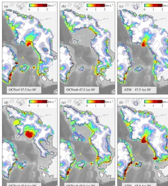
Figure 7.Simulated EIS at the end of a stadial period(a–c)and at the end of an interstadial period(d–f)for the OCNsrf(a, d), OCNsub(b, e) and ATM(c, f)experiments. Shaded colors show ice velocities (in kilometers per annum). The ice thickness contours are plotted for every 500 m with the grounding-line position shown using a black line. The 500 m depth contour is shown using a white line. The periods represented here corresponds to the stadial and interstadial periods prior and posterior to DO 12 (ca. 47 kyr BP), respectively.
shifting to pronounced stadial periods (as in ca. 44 kyr BP) favors the penetration of warm subsurface waters that in-crease basal melting enough to produce an ice-sheet retreat in the northeastern part in spite of the enhanced positive sur-face mass balance (Figs. 5, 6). When considering the atmo-sphere and the subsurface ocean forcing together in ALLsub,
these competing processes translate into a smaller amplitude of millennial-scale EIS changes compared with the case with surface ocean forcing (ALLsrf). Furthermore, declines of the
EIS can be observed both during the beginning of intersta-dial periods and during pronounced staintersta-dial periods in ALLsub
(Figs. 5, 6).
Focusing on the OCN and ATM simulations separately fa-cilitates isolating the effects of the ocean on this complex pattern. To this end, the simulated ice-sheet distribution and velocities of OCNsrf, OCNsuband ATM are shown in Fig. 7
for the period around DO-event 12, at ca. 47 kyr BP. As
ex-pected, OCNsrfshows a widespread retreat both in the
north-east and the southwest of the EIS from the stadial to the in-terstadial period (Fig. 7d). This is accompanied by an ac-celeration of the Bjørnøyrenna Basin due to its grounding-line thinning and retreat (Fig. 7a, d). OCNsubpresents a
col-lapsed Bjørnøyrenna Basin during the stadial period previous to DO-event 12 due to enhanced basal melting from warmer subsurface waters. The transition to the interstadial period favors a slight regrowth of this northeastern part of the EIS due to decreased basal melting, while its southwestern sec-tion slightly retreats (Fig. 7b, c)
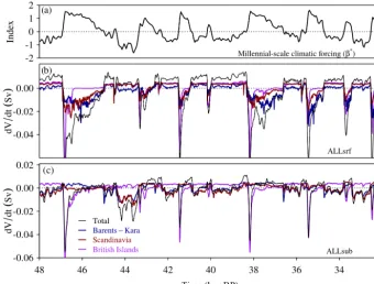
Figure 8.MIS 3 period.(a)Temporal component of the millennial-scale climatic forcing (β? index), and the contribution of the different regions to ice volume variations (Sv) in the simulations considering all forcings, with (b)corresponding to the surface oceanic forcing (ALLsrf) and(c)to the subsurface oceanic forcing (ALLsub). The geographical domains of the different regions are highlighted in Fig. 2.
ice volume reduction of the EIS in ATM during interstadi-als is due to the positive SAT anomaly, which leads to en-hanced ablation in the southwestern part of the EIS (Fig. S5). In turn, reduced SATs during stadials allow the regrowth of the ice sheet up to the continental margin of the Nordic seas. The more active dynamic response of the EIS in the OCN simulations can be attributed to the increase in oceanic tem-peratures by 2–4◦C (Fig. 3) within the margins of the ice sheet during interstadial (in the case of OCNsrf) and stadial
(OCNsubcase) periods, which translates into enhanced basal
melting at the margins of the EIS. The southwestern sector of the EIS also responds to the warmer SSTs, even displaying a larger reduction of ice volume than in ATM (Fig. 7).
The spatial patterns shown in Fig. 7 are representative of the ice-sheet response during all other stadial–interstadial transitions. In OCNsrf, the EIS reacts to every abrupt surface
warming with a substantial ice-flow acceleration, especially in the Bjørnøyrenna Basin (Figs. 7, 8, 9). Ice shelves that are present during stadial periods suddenly retreat during DO-events and in combination with enhanced basal melting favor thinning and retreat of the grounding line that translate into large iceberg discharges of up to ca. 0.06 Sv. In OCNsub, ice
velocities in the Bjørnøyrenna Basin increase during stadi-als, when enhanced basal melting erodes the grounding line and favors its retreat. Peaks in calving are recorded accord-ingly during pronounced stadial periods (Fig. 10). However, these peaks are of smaller amplitude than in OCNsrf. This
can be explained by the fact that, along the coast of Eura-sia, the amplitude of the simulated SST anomalies used to compute basal melting in OCNsrf is larger than the
subsur-face temperature anomalies in OCNsub, as the basal melt was
calculated by using ocean temperature at a fixed depth, either at the surface or at the subsurface. Also, transitions to stadi-als are usually more gradual than transitions to interstadistadi-als; thus, in this case, the incursion of warmer (subsurface) wa-ters occurs in a smoother manner. High velocities reach their maxima at the end of the stadial and beginning of the intersta-dials. However, the latter are not accompanied by an increase in calving due to the fact that ice shelves are expanding and thickening during this period thanks to reduced basal melting (Fig. 10). In general, the extension of ice shelves is greatly re-duced during periods of enhanced basal melting (Figs. 9, 10), with no large unconfined ice shelves surviving during these episodes. Some thinner ice shelves remain, in spite of the enhanced basal melting, thanks to an increase in advection from the Bjørnøyrenna ice stream triggered by a grounding-line retreat (Fig. 7).
3.3 Grounding-line dynamics
indi-Figure 9.MIS 3 period. Temporal component of the millennial-scale climatic forcing (β?index), ice velocities in the Bjørnøyrenna Basin (calculated as mean values over the entire basin in kilometers per annum), calving rate (Sv) and ice-shelf area (103km2) in the OCNsrf simulation.
cator for characterizing the dynamic behavior of the marine part of the EIS. Inspection of the temporal evolution of the grounding-line position in OCN simulations confirms that ice dynamics control the majority of ice-volume variations in the EIS as opposed to the SMB processes involved in ATM (Fig. 11). The migration of the grounding line through time has been characterized by means of an index (µ) that weighs the proportion of non-grounded points in the region of the Bjørnøyrenna Basin:
µ(t)=
1−Ng(t) N
·100, (21)
whereNg(t) represents the evolution of the number of points
of grounded ice within a fixed area ofN points in the Bar-ents Sea region defined over the black square highlighting the Bjørnøyrenna Basin shown in Fig. 2. Note that other met-rics are also possible; the same metric has been used in other studies in different domains such as Antarctica (Blasco et al., 2018).
Thus, an increase (decrease) in µindicates a retreat (ad-vance) of the grounding line. While in ATM µ barely changes Fig. 11), OCN runs show a large dynamic behavior of the basin. In OCNsrf,µreflects a synchronous evolution
of the grounding-line position and the oceanic forcing, with major retreats coinciding with interstadial states (Fig. 11). Conversely, the Bjørnøyrenna Basin is generally much closer to a full retreat in OCNsubduring stadials due to a larger
pen-etration of warm subsurface waters (Fig. 3; OCNsub)
com-pared to the surface waters (Fig. 3; OCNsrf). However, the
grounding line is able to advance and reach Svalbard during episodes of reduced basal melting at the interstadials.
The direct coupling between the oceanic forcing and the response of the Bjørnøyrenna ice stream is also evident from the relatively high negative correlation (r' −0.9) found be-tween µ and ice thickness in this area (Fig. 11). A lo-cal thinning of the grounding line produced by a warmer ocean triggers its retreat and starts the propagation of the dynamic imbalance of the ice stream. The propagation of a change in the surface slope occurs almost instantaneously at these timescales (with a typical propagation speed of about 10 km a−1). This chain of processes explains the tightened linear relationship between the Bjørnøyrenna Basin thickness and the grounding-line position,µ. Although a grounding-line retreat (advance) of the grounding grounding-line in this region produces an acceleration (deceleration) of the ice streams, its linear relationship is less obvious than that for ice thick-ness (Fig. 11c). This is explained by the fact that ice-stream velocities lag the grounding-line imbalance due to the char-acteristic time for the kinematic wave to propagate along the ice streams of the whole basin (typically of∼1 km a−1).
As a consequence of the destabilization of the ice sheet, important ice-volume variations observed in the northeastern part of the EIS during millennial-scale climatic transitions, which added to the minor contribution of the southwestern retreat (Fig. 8), result in fluctuations of more than 4 m SLE in OCNsrf, up to 2.5 m in OCNsuband ca. 1 m in ATM (Fig. 4).
Figure 10.MIS 3 period. Temporal component of the millennial-scale climatic forcing (β?index), ice velocities in the Bjørnøyrenna Basin (calculated as mean values over the entire basin in kilometers per annum), calving rate (Sv) and ice-shelf area (103km2) in the OCNsub simulation.
Figure 11.Dynamic behavior of the EIS during millennial-scale climatic transitions for the OCNsrf, OCNsuband ATM experiments. Dis-placement of the grounding line in the Bjørnøyrenna Basin(b)in response to the climaticβ?forcing(a). The evolution of the grounding-line position is shown for OCNsrf(blue), OCNsub(red) and ATM (gold). The migration of the grounding line has been characterized as an index µ(t) that represents the evolution of the number of points of grounded iceNg(t) over a fixed area ofN points in the Barents Sea region, defined over the black square highlighting the Bjørnøyrenna Basin shown in Fig. 2. Increasing values ofµindicate grounding-line retreat. (b)OCNsrfscatterplot diagram showing the relationship between mean ice thicknessHin the region of the Bjørnøyrenna Basin andµ(light blue diamonds) as well as the relationship between ice-stream velocitiesvin the same region andµ(purple circles).
with different κ parameters between 1 and 10 m a−1K−1, i.e., bracketing our standard case of κ=5 m a−1K−1. This choice reflects the inferences based on measurements made on Antarctic ice shelves that a variation of 1 K in the effective oceanic temperature changes the melt rate by ca. 10 m a−1
(Rignot and Jacobs, 2002; Shepherd et al., 2004). A robust response of the EIS is found, with a more reactive EIS
amplitude than the one induced by the atmosphere provided thatκ >2 m a−1K−1(see Fig. S3 of the Supplement).
4 Discussion
Our results suggest a highly dynamic Eurasian ice sheet at millennial timescales largely responding to changes in the ocean temperatures. Some authors (e.g., Gudlaugsson et al., 2013) present the marine based Barents–Kara complex as an analogue for the present-day West Antarctic ice sheet for which bedrock topography is a major control for stability. We have shown, in this sense, that the Bjørnøyrenna Basin is highly susceptible to changes in the oceanic temperatures.
Our results indicate that the timing of the response with respect to changes registered in Greenland (i.e., their occur-rence during stadials or interstadial) depends, however, on whether the surface or the subsurface of the ocean is con-sidered as the relevant forcing of the ice sheet. Recently, IRD peaks of Fennoscandian origin reported from a high-resolution marine sediment core from the Norwegian Sea in-dicate the presence of more frequent IRD deposition and thus calving during interstadials than during stadials (Dokken et al., 2013). This result has been corroborated in a compi-lation of new and previously published data (Becker et al., 2017) clearly showing that the IRD deposition increases within interstadials within MIS 3. The coeval deposition of carbonate-rich, sorted fine sands and near-surface warming suggests the presence of Atlantic water along the margin, and is interpreted by the authors as the effects of winnow-ing due to an intensified AMOC durwinnow-ing interstadials. This interpretation results in concordance with our results when considering the surface waters as the oceanic forcing. Thus, this agreement would play in favor of considering that the EIS was primarily responding to changes in the surface of the ocean along the southwest EIS (Irish/Scottish margin) at least.
An out-of-phase relationship is found in the dynamic re-sponse of the EIS when forcing the ice-sheet model with the millennial-scale simulated surface and subsurface tempera-ture anomalies. This behavior results from the roughly oppo-site sign of their spatial forcing patterns in the Nordic seas. This pattern has been found to be robust in a number of mod-els but its details could well be model dependent, and, in par-ticular, dependent on the precise location of the convection sites affected (e.g., Brady and Otto-Bliesner, 2011; Mignot et al., 2007; Montoya and Levermann, 2008; Shaffer et al., 2004; Flückiger et al., 2006).
Our results also provide a mechanism to explain the per-vasive presence of IRD in the North Atlantic during MIS 3, both during stadials and interstadials, and originating both in the LIS and the EIS. During stadials, the simultaneous ap-pearance of IRD across the wider North Atlantic Ocean can be explained by the buildup of subsurface heat in the high-latitude North Atlantic leading to increased iceberg calving
in the presence of large, thick ice shelves, and lower surface temperatures allowing for wider dispersal of icebergs (Barker et al., 2015). According to our results interstadials could lead to enhanced calving of the EIS through oceanic surface sub-glacial melting as a result of the warmer surface conditions and relatively shallow grounding lines of this ice sheet.
The identification of IRD layers with increased calving through ice-sheet instabilities must be taken with caution, as it is based on several untested assumptions (Clark and Pisias, 2000): (i) the delivery of IRD to a specific site is caused solely by iceberg calving, versus transport by sea ice; (ii) an increase in IRD represents an increase in the iceberg flux, versus a greater amount of debris incorporated at the base of the ice sheet that delivers the icebergs, or a greater distance of iceberg transport; (iii) the amount of IRD carried by all the icebergs is similar, therefore assuming a direct relation-ship between IRD concentration and iceberg flux. However, the former assumptions have not been confirmed and, thus, the calving–IRD relationship might not be so direct. In addi-tion, ocean temperatures affect melting of icebergs and thus their release of IRD. Variations in ocean temperatures can al-ter the IRD released by an iceberg at a certain site, causing variations in IRD deposition even for a constant amount of icebergs produced at the source.
Furthermore, it has been suggested (Pollard et al., 2015) that the ice front can suffer dramatic calving in vertical ter-mini glaciers due to the so-called cliff instability mechanism. This process is not parameterized in our model. We believe its inclusion would, if anything, amplify the simulated re-sponse of the EIS to the ocean forcing. Nonetheless, the ne-cessity of including this phenomenon in ice-sheet models has recently been contested (Edwards et al., 2019).
Our experimental setup is not intended to match the pa-leorecord, but to provide insight into the response of the EIS to millennial-scale variability. The EIS variations sim-ulated here represent the upper-end amplitude of potential responses during the whole glacial cycle, due to its large size. Extending the study to cover the whole LGP requires the consideration of orbital variability as part of the forcing (see the Supplement). In this case, the EIS is smaller during the mildest phase of MIS 3, thus limiting its contact with the ocean and the production of iceberg discharges (Fig. S6).
Furthermore, our results depend somewhat on the partic-ular SAT and oceanic temperature anomaly patterns simu-lated by our climate model, the magnitudes of the resulting forcing, and the initial size of the simulated EIS. As the re-sponse to the ocean has been found to be dominant, a larger ice sheet, with more developed ice shelves and thus more ex-posed to the ocean would be prone to suffer stronger basal melting; destabilization of ice shelves could therefore result in a more dynamic ice sheet with larger calving peaks. A smaller ice sheet would consequently only be affected by at-mospheric forcing. The use of different atat-mospheric realiza-tions is subject to the availability of climate simularealiza-tions with different models for the three climate states needed: glacial (stadial), present and interstadial. The latter is only available for a reduced number of models. This makes the assessment of this issue difficult in the present study. Assessing the sensi-tivity to these features should be in the scope of future work, and illustrates the need for carrying out new simulations of both the interstadial and the stadial states using more sophis-ticated climate models. Nonetheless, our results indicate that the ocean is the major driver of the EIS ice-volume changes during MIS 3. Note that the temporal index used is the same for the atmosphere and the ocean, and the amplitude is given by an ocean general circulation model simulation of two dif-ferent oceanic states mimicking stadial and interstadial pe-riods. We then translate those fields into ablation (via PDD, for which the uncertainty has been extensively explored) and into basal melting (using a linear equation). It is conceiv-able that our synthetic oceanic temperature forcing is larger than that deduced from reconstructions in certain locations, which range from 4 to 10 K (Dokken et al., 2013; Martrat et al., 2004; Rasmussen et al., 2016). However, the possible uncertainty in the temperature forcing is subsumed in theκ index which in our case varies between 1 and 10 m a−1K−1. These values are in the range (or even below in most cases) of those suggested by data in Antarctica (Rignot and Jacobs, 2002). Note, in particular, that even from mid-values ofκof
5 m a−1K−1the response to the ocean is already of greater amplitude than that to the atmosphere, making our main con-clusions robust.
For the sake of simplicity, and following up from previ-ous work (Alvarez-Solas et al., 2011a, 2013), in this study we calculated the basal melt using ocean temperature at a fixed depth, either at the surface or at the subsurface. Using the three-dimensional temperature provided by the climate model at the local ice-shelf depth that can evolve in time as the ice-shelf thickness varies would have been more realistic and should be in the scope of future work.
Finally, our study lacks bidirectional coupling between the ice sheet, the atmosphere and the ocean. Eventually the goal is to investigate this matter with fully coupled climate–ice-sheet models.
Circumpolar Deep Water (CDW) in Antarctic ice-shelf cavi-ties, and thereby submarine melting (Naughten et al., 2018). This mechanism is also found in a coupled climate model in-cluding an eddying ocean component (Goddard et al., 2017). Thus, changes in ocean water temperatures appear to be key in driving ice-sheet changes in both the past and future.
Meltwater discharge from the EIS and other ice sheets sur-rounding the Nordic seas is often implied as a cause of ocean instabilities (e.g., Broecker et al., 1985; Clark et al., 2002; Ganopolski and Rahmstorf, 2001; Rasmussen and Thomsen, 2013; Schmittner et al., 2002). The same would be the case for iceberg discharges. This issue is beyond the scope of this study; its assessment would require investigating the impact of these freshwater perturbations in deep water formation and the AMOC. Again, proper assessment requires the use of a coupled climate–ice-sheet model.
5 Conclusions
We have investigated the response of the EIS to millennial-scale climate variability associated with DO-events through a series of simulations with a three-dimensional, hybrid ice-sheet model that represents inland ice flow under the SIA and floating ice shelves and ice streams through the SSA. The model also includes an explicit grounding-line treatment, a simple basal melting parameterization that depends linearly on the ocean temperature anomalies and calving via a dou-ble criterion on ice thickness and advection at the ice front. The model makes use of an off-line forcing method that sepa-rately accounts for orbital- and millennial-scale climate vari-ability during the LGP, improving the representation of the latter (Banderas et al., 2018). Atmospheric and ocean forc-ings associated with millennial-scale variability were consid-ered both separately and together.
Oceanic forcing was considered both at the surface and at the subsurface. The timing of the response with respect to changes registered in Greenland depends on whether the sur-face or the subsursur-face of the ocean is considered as the rele-vant forcing of the ice sheet. A quasi-antiphase relationship is found in these two cases. This behavior can be explained by the fact that ocean waters at the subsurface warm (cool) dur-ing episodes of reduced (enhanced) convection at the Nordic seas as a result of variations in the AMOC strength.
Separating the effects of atmospheric and oceanic forc-ing durforc-ing the glacial period has allowed us to quantify the contribution of each to EIS variability. Atmospheric forcing during stadial–interstadial transitions has a modest effect on the ice sheet, which is a consequence of the largest SMB changes being confined to southwestern sector of the EIS, where the forcing is strongest. In contrast, the oceanic forc-ing has a larger effect, through changes in the ice dynamics in the Bjørnøyrenna Basin on the EIS. Ocean warming is able to induce a retreat of grounded ice in this part of the EIS through dynamic processes. As a consequence, significant
ice-volume variations result during millennial-scale climatic transitions. Added to the smaller contribution of the south-western retreat, this results in sea-level changes on the order of several meters. Sensitivity experiments for different val-ues of the oceanic heat coefficient parameter show that this is a robust response of the model.
Thus, our results support the existence of a highly dy-namic EIS during the LGP. They suggest an important role of oceanic melt forcing through changes in the ocean circula-tion in controlling the ice-stream activity. A number of stud-ies have considered the interaction between ocean circulation changes and ice-sheet dynamics as a plausible mechanism to explain iceberg discharges from the LIS associated with H-events. For example, subsurface oceanic warming during stadials in response to reduced North Atlantic deep water for-mation (Alvarez-Solas et al., 2010; Flückiger et al., 2006; Mignot et al., 2007; Shaffer et al., 2004) has been shown to be capable of producing large discharges from the LIS, in-duced by enhanced basal melting rates (Marcott et al., 2011; Álvarez-Solas et al., 2011b). The satisfactory agreement be-tween the simulated calving and North Atlantic marine IRD records provides strong support for this mechanism (Alvarez-Solas et al., 2013), recently proposed to be modulated by isostatic adjustment (Bassis et al., 2017). The evaluation of the impact of these Northern Hemisphere discharges on the oceanic circulation and their effects on the triggering mecha-nism of DO-events require the use of a coupled climate–ice-sheet model. Nonetheless, it has recently been shown that the typical oceanic cooling registered in sediment cores of the North Atlantic during stadials occurs before the arrival of the icebergs to these same cores (Barker et al., 2015). In this sense, iceberg discharges from the Laurentide and the Eurasian ice sheets are seen as potential amplifiers but not as active elements in the triggering of millennial-scale vari-ability. In combination with these studies, our results sup-port the potential of Northern Hemisphere ice sheets to act to glacial abrupt climate changes. Additionally, our re-sults highlight the need for stronger constraints on the lo-cal North Atlantic behavior in order to shed light on the Northern Hemisphere ice sheet’s glacial dynamics. As the ocean plays a major role during abrupt ice sheet changes, the model’s treatment of grounding-line dynamics is a key issue. Finally, this represents one of the first attempts to sim-ulate both oceanic and atmospheric impacts on ice sheets as-sociated with abrupt climate changes. Investigating this is-sue further with higher resolution and exploring the effect of the underlying uncertainties in ice-sheet and grounding-line dynamics is of uttermost interest and in the scope of future work.
are available at https://doi.org/10.17605/OSF.IO/3KFUA (Alvarez-Solas, 2019).
Supplement. The supplement related to this article is available online at: https://doi.org/10.5194/cp-15-957-2019-supplement.
Author contributions. JAS performed the simulations. All au-thors contributed to developing of the method, analysing the results and writing the paper.
Competing interests. The authors declare that they have no con-flict of interest.
Acknowledgements. This work was funded by the Spanish Min-isterio de Economía y Competitividad (MINECO) through project MOCCA (Modelling Abrupt Climate Change, grant no. CGL2014-59384-R). Rubén Banderas was funded by a PhD thesis grant from the Universidad Complutense de Madrid. Alexander Robinson is funded by the Marie Curie Horizon 2020 project CONCLIMA (grant no. 703251). Part of the computations undertaken in this work were performed in EOLO, the HPC of Climate Change of the Inter-national Campus of Excellence of Moncloa, funded by MECD and MICINN. This is a contribution to CEI Moncloa. We are grateful to Catherine Ritz for providing the GRISLI code.
Review statement. This paper was edited by Hugues Goosse and reviewed by three anonymous referees.
References
Åkesson, H., Morlighem, M., Nisancioglu, K. H., Svendsen, J. I., and Mangerud, J.: Atmosphere-driven ice sheet mass loss paced by topography: Insights from modelling the south-western Scan-dinavian Ice Sheet, Quaternary Sci. Rev., 195, 32–47, 2018. Alley, R. B., Clark, P. U., Huybrechts, P., and Joughin, I.:
The deglaciation of the Northern Hemisphere: a global perspective, Annu. Rev. Earth Pl. Sc., 27, 149–182, https://doi.org/10.1146/annurev.earth.27.1.149, 1999.
Alvarez-Solas, J.: Glacial Fennoscandian GRISLI-UCM simula-tions, https://doi.org/10.17605/OSF.IO/3KFUA, 2019.
Alvarez-Solas, J., Charbit, S., Ritz, C., Paillard, D., Ramstein, G., and Dumas, C.: Links between ocean temperature and ice-berg discharge during Heinrich events, Nat. Geosci., 3, 122–126, https://doi.org/10.1038/ngeo752, 2010.
Alvarez-Solas, J., Charbit, S., Ramstein, G., Paillard, D., Dumas, C., Ritz, C., and Roche, D. M.: Millennial-scale oscillations in the Southern Ocean in response to atmospheric CO2increase, Global Planet. Change, 76, 128–136, 2011a.
Álvarez-Solas, J., Montoya, M., Ritz, C., Ramstein, G., Char-bit, S., Dumas, C., Nisancioglu, K., Dokken, T., and Ganopol-ski, A.: Heinrich event 1: an example of dynamical ice-sheet reaction to oceanic changes, Clim. Past, 7, 1297–1306, https://doi.org/10.5194/cp-7-1297-2011, 2011.
Alvarez-Solas, J., Robinson, A., Montoya, M., and Ritz, C.: Iceberg discharges of the last glacial period driven by oceanic circulation changes, P. Natl. Acad. Sci. USA, 110, 16350–16354, 2013. Amante, C. and Eakins, B. W.: ETOPO1 1 Arc-minute Global
Relief Model: Procedures, Data Sources and Analysis, NOAA, USA, https://doi.org/10.7289/V5C8276M, 2009.
Anderson, J. B., Shipp, S. S., Lowe, A. L., Wellner, J. S., and Mosola, A. B.: The Antarctic Ice Sheet during the Last Glacial Maximum and its subsequent retreat history: a review, Qua-ternary Sci. Rev., 21, 49–70, https://doi.org/10.1016/S0277-3791(01)00083-X, 2002.
Andreassen, K. and Winsborrow, M.: Signature of ice streaming in Bjørnøyrenna, Polar North Atlantic, through the Pleistocene and implications for ice-stream dynamics, Ann. Glaciol., 50, 17–26, https://doi.org/10.3189/172756409789624238, 2009.
Asay-Davis, X. S., Jourdain, N. C., and Nakayama, Y.: Develop-ments in Simulating and Parameterizing Interactions Between the Southern Ocean and the Antarctic Ice Sheet, Current Climate Change Reports, 3, 316–329, https://doi.org/10.1007/s40641-017-0071-0, 2017.
Bamber, J. L., Griggs, J. A., Hurkmans, R. T. W. L., Dowdeswell, J. A., Gogineni, S. P., Howat, I., Mouginot, J., Paden, J., Palmer, S., Rignot, E., and Steinhage, D.: A new bed el-evation dataset for Greenland, The Cryosphere, 7, 499–510, https://doi.org/10.5194/tc-7-499-2013, 2013.
Bamber, J. L., Layberry, R. L., and Gogineni, S.: A new ice thick-ness and bed data set for the Greenland ice sheet: 1. Measure-ment, data reduction, and errors, J. Geophys. Res.-Atmos., 106, 33773–33780, 2001.
Banderas, R., Alvarez-Solas, J., Robinson, A., and Montoya, M.: An interhemispheric mechanism for glacial abrupt climate change, Clim. Dynam., 44, 2897–2908, https://doi.org/10.1007/s00382-014-2211-8, 2015.
Banderas, R., Alvarez-Solas, J., Robinson, A., and Montoya, M.: A new approach for simulating the paleo-evolution of the North-ern Hemisphere ice sheets, Geosci. Model Dev., 11, 2299–2314, https://doi.org/10.5194/gmd-11-2299-2018, 2018.
Barker, S., Chen, J., Gong, X., Jonkers, L., Knorr, G., and Thornal-ley, D.: Icebergs not the trigger for North Atlantic cold events, Nature, 520, 333–336, https://doi.org/10.1038/nature14330, 2015.
Bassis, J. N., Petersen, S. V., and Mac Cathles, L.: Heinrich events triggered by ocean forcing and modulated by isostatic adjust-ment, Nature, 542, 332–334, 2017.
Becker, L. W., Sejrup, H. P., Hjelstuen, B. O., Haflidason, H., and Dokken, T. M.: Ocean-ice sheet interaction along the SE Nordic Seas margin from 35 to 15 ka BP, Mar. Geol., 402, 99– 117, https://doi.org/10.1016/j.margeo.2017.09.003, 2017. Beckmann, A. and Goosse, H.: A parameterization of ice
shelf-ocean interaction for climate models, Ocean Model., 5, 157–170, 2003.
Bentley, M. J., Cofaigh, C. O., Anderson, J. B., Conway, H., Davies, B., Graham, A. G., Hillenbrand, C.-D., Hodgson, D. A., Jamieson, S. S., Larter, R. D., and Mackintosh, A.: A community-based geological reconstruction of Antarctic Ice Sheet deglaciation since the Last Glacial Maximum, Quaternary Sci. Rev., 100, 1–9, 2014.