Response of the PUI Distribution To Variable Solar Wind Conditions

(1)

University of New Hampshire

University of New Hampshire Scholars' Repository

Master's Theses and Capstones Student Scholarship

Spring 2018

Response of the PUI Distribution To Variable Solar

Wind Conditions

Jonathan Slade Bower

University of New Hampshire, Durham

Follow this and additional works at:https://scholars.unh.edu/thesis

This Thesis is brought to you for free and open access by the Student Scholarship at University of New Hampshire Scholars' Repository. It has been accepted for inclusion in Master's Theses and Capstones by an authorized administrator of University of New Hampshire Scholars' Repository. For more information, please [email protected].

Recommended Citation

Bower, Jonathan Slade, "Response of the PUI Distribution To Variable Solar Wind Conditions" (2018).Master's Theses and Capstones. 1193.

(2)

Response of the Pickup Ion

Distribution to Variable Solar Wind

Conditions

By:

Jonathan

_Bower

BS, University of New Hampshire, 2015

THESIS

Submitted to the University of New Hampshire

in Partial Fulfillment of the Requirements for

the Degree of

Master of Science

in

Physics

(3)

This thesis has been examined and approved in partial fulfillment of the requirements for the degree of Master of Science in Physics by:

Dr. Eberhard M¨obius, Professor Emeritus, Thesis Advisor, Department of Physics and Space Science (EOS)

Dr. Martin Lee, Professor Emeritus, Physics and Space Science

Dr. John Dawson, Professor Emeritus, Physics

May 3, 2018

(4)

1 Introduction

Pickup Ions are created when neutrals moving through a magnetized plasma are ionized through photo-ionization, electron impact or charge exchange [Schwadron, 1998]. Once ionized, they experience a Lorentz force and undergo cyclotron motion, with a guiding center moving with the plasma. In the plasma’s reference frame the ions gyrate around the magnetic field lines, and depending on the direction of their initial velocity, they will move freely along the magnetic field as well.

In the Heliosphere, pickup ions (PUI) are generated from several different interplan-etary and interstellar neutral sources which are ionized by the Sun’s radiation or inter-action with the solar wind, and are picked up by the frozen-in interplanetary magnetic field (IMF). Once implanted in the solar wind the newly ionized particles are convected radially outward, typically occupying a velocity range from 0 km/s to twice the solar wind speed, associated with the ion’s cyclotron motion. Immediately after injection, the velocity distribution of the PUI population is highly anisotropic and forms a torus in velocity space [Kallenbach et al., 2000]. The population undergoes cooling processes (SW expansion and decreases in the IMF field strength) and achieves isotropy through scattering (pitch angle scattering and turbulence) [Kallenbach et al., 2000].

(7)

Figure 1: Basic structure of the Heliosphere, formed by the dynamic solar wind and the partially ionized ISM and their embedded magnetic fields [Frazier and Garner, 2017]

about the SW interaction with the ISM is continuously translated through the medium, forming the Heliosheath, a region where the wind is slowed, compressed and turbulent [Axford and Suess, 1994]. As the solar wind slows and continues to expand, it eventually pressure balances with the interstellar medium and the flow is halted. This boundary is known as the Heliopause, beyond which lies the interstellar medium.

Scientists believe this boundary was measured directly by Voyager 1 in May of 2012 when it detected a rapid increase in the galactic cosmic ray flux, in conjunction with a decrease in the anomalous cosmic ray flux [Kallenbach et al., 2000]. Essentially, because of this interaction, charged particle populations are unable to penetrate far enough into the heliosphere to be measurable at 1AU. The consequence being that we must rely on direct observation of the neutral gas which penetrates almost unimpeded into the heliosphere. We diagnose the neutral gas in the inner heliosphere through solar UV backscattering, PUI measurement and direct neutral imaging [Moebius et al., 2004].

(8)

abundance, while He and Ne survive much more readily due to their high ionization potential [Kallenbach et al., 2000]. At Earth’s orbit, He has the highest density of all the neutrals, making it the easiest to observe. The first observations of interstellar pickup ions were in fact He, measured by the SULEICA instrument on the AMPTE spacecraft [Moebius et al., 1985].

Because the solar wind plasma is largely collisionless, once injected, PUIs are only acted on by fluctuations in the local magnetic fields. These fluctuations can scatter the PUI populations and cause energy diffusion, leading to transport effects, such as pitch angle scattering, cooling and acceleration. Additionally, the expansion of the solar wind will result in a decreased magnetic field strength thus cooling the PUIs further [Saul et al., 2004]. If we can understand these transport effects and describe them accordingly we can build the PUI velocity distribution function (VDF) such that we can determine the underlying parameters of the PUI source population. The determination of physical parameters of the ISM has been one of the important scientific goals of several satellite missions in recent years, and is of continued interest to the scientific community.

(9)

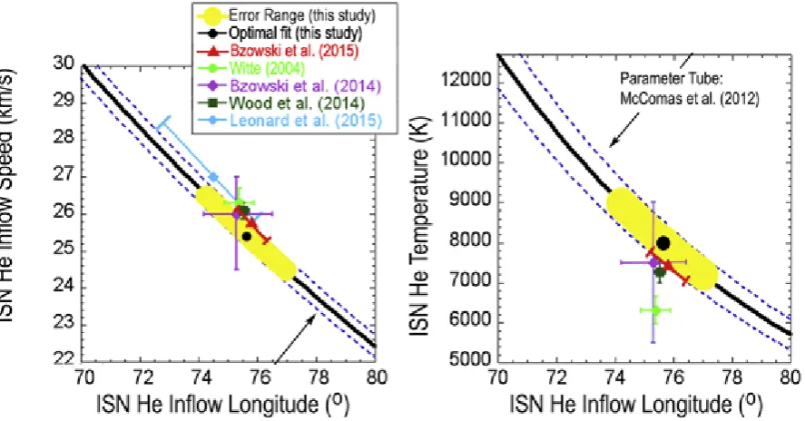
Figure 2: IBEX’s functional relationship showing coupling between the inflow velocity and longitude (left) and the temperature and longitude (right). [Schwadron et al., 2015]

along the tube.

Independent determinations of individual parameters can be used to break the de-generacy and drastically increase the accuracy of all coupled parameters. Here we will discuss how He+ PUI measurements taken aboard the STEREO A satellite, can be used to determine the inflow longitude of the ISM to a great degree of accuracy and thereby break the degeneracy of the IBEX observations. This method, developed in Moebius et al. [2015], utilizes the variation of the radial neutral flow speed as a function of eclip-tic longitude to determine the bulk neutral inflow direction. The longitudinal velocity variation of the neutrals manifests itself in the PUI velocity distribution by increasing or decreasing PUI cutoff (the point on the PUI VDF where the phase space density sharply decreases). Since the PUI cutoff is dependent on the radial neutral velocity at injection, the cutoff is increased upwind where the neutral flow is running into the solar wind, and decreased downwind where the neutral flow is running with the solar wind. Thus measuring the PUI cutoff as a function of ecliptic longitude and finding the max cutoff location will result in the neutral flow direction.

(10)

(a) (b)

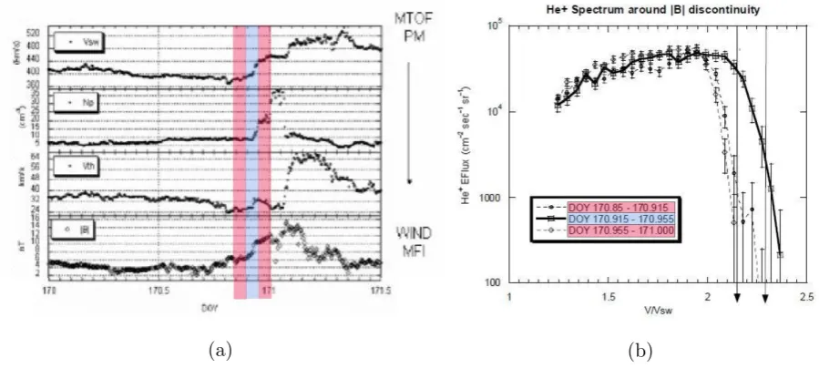
Figure 3: Effect of a SW compression on the PUI VDF as seen by SOHO CELIAS CTOF. (a) shows solar wind parameters evolving across single compression region, where red designates regions before and after the compression and blue designates the region under compression. (b) shows the velocity distribution function, before, during and after the compression has passed. [Saul et al., 2004]

cooling. These interactions were first observed in Saul et al. [2004], where several com-pressions in the solar wind parameters were observed, resulting in positive cutoff shifts in the PUI VDFs. One such compression is shown in Figure 3. Here the compression is identified in blue, PUI VDFs are integrated in three time ranges, before, during and after the compression, and their cutoffs are identified. Prior to the compression arrival the PUI VDF has a sharp cutoff at w= 2vsw, during the compression, the PUI cutoff was shown

to be shifted to higher velocities, signifying a heating of the embedded PUIs. After the rapid increase in solar wind velocity is over, the PUI cutoff returns to pre-compression levels. All of this takes place over the course of hours, showing that these SW velocity changes can manifest themselves as large variations in the PUI cutoff.

(11)

behavior in compression regions and interplanetary shocks, and to develop criteria to remove or correct for these effects in the determination of the ISN flow direction.

(12)

2 Generation and Transport of PUI’s

In order to have a functional understanding of the effects of PUI transport we need some background information about PUI origins, their velocity distribution functions and how they evolve under different solar wind conditions.

2.1 PUI Generation and Neutral Sources

As was briefly discussed, PUIs begin as neutral particles sourced from populations in the partially ionized interstellar medium, interplanetary dust, and planetary, lunar and cometary atmospheres. For this study, we will focus on PUIs generated from interstellar neutrals. The interplanetary magnetic field, frozen into the solar wind, prevents the ionized portion of the ISM from penetrating the heliosphere. As the solar system moves through interstellar space the neutral population in the ISM is able to flow unimpeded through the essentially collisionless solar wind and part of this population is thus readily available to be measured at 1au. This neutral flow is primarily comprised of H and He, but also contains trace amounts of, O, N and Ne when compared to H [Herbst, 1995]. As the flow passes through the heliosphere, neutrals are lost to ionization processes, namely photoionization and charge exchange collision, creating an ionization cavity close to the Sun. H, O and N have relatively low ionization potentials compared to He and Ne, resulting in a higher portion of these particles lost to ionization. This means that He and Ne exist in higher percentages at Earth’s orbit. Because He is the second most abundant neutral in the ISM, its survivability makes it the best test particle at Earth [Herbst, 1995]. The physical parameters of He held consensus values of nHe = 0.015±

0.002cm−3_,_v

He = 26.3±0.4km/sand THe = 6300±390◦K [Moebius et al., 2004]. IBEX

measurements have since shown that this temperature value is an underestimation, where

THe = 8710 + 440/−80◦K for vHe = 26.3 [Moebius et al., 2015a]. A certain portion of

the ions from the outer heliosphere undergo charge exchange to produce neutrals, some of these particles will yield velocity vectors that bring them into the inner heliosphere, generating a secondary neutral flow [Moebius et al., 2009]. The bulk of these particles charge exchange in the heliosheath, and as such, retain the velocity distribution of the compressed plasma. These secondary neutrals have a slower bulk velocity, but a higher temperature than the interstellar neutrals [Moebius et al., 2009].

(13)

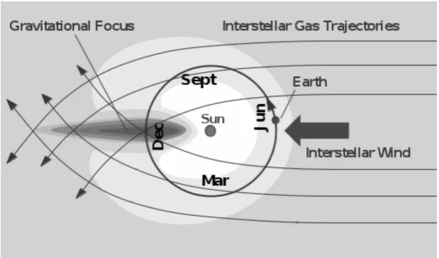
Figure 4: Schematic view of primary neutral density structures and neutral particle trajectories. The Ionization cavity is seen upwind in white near the Sun where neutral particles are deplete. The gravitation focusing cone is seen downwind in gray where the neutral density is high [Moebius et al., 1999].

downwind. The ionization cavity coupled with the neutral particle acceleration result in the characteristic density structure seen in Figure 4. Here, sample trajectories of the neutral He are shown bending around the Sun, creating the gravitational focusing cone downwind. The variation of the neutral radial velocity manifests itself in the velocity distribution of PUIs, and can be exploited to measure the inflow direction.

(14)

Figure 5: Schematic view of the velocity distribution in the spacecraft frame for PUI injected with a perpendicular magnetic field (left) and a near parallel magnetic field (right) [Saul et al., 2004]. The x axis is associated with the Sun-spacecraft line or the radial direction.

2.2 PUI Gyration

The Lorentz force is fundamentally the most important transport effect that governs PUI motion as well as the least complex to describe. In the simplest terms the motion of the PUIs can be approximated by looking at the assumed stationary electromagnetic fields in the solar wind.

F =q(E~ +~v×B~) (1)

Where E~ is the local convective electric field, generated by the moving SW. B~ is the magnetic field vector and ~v is the particle velocity. Transforming into the solar wind frame gives an initial velocity of the PUIs ~v =~vneutral −~vsw. Usually, at injection, the

particle velocity is assumed to be near zero in the inertial frame which gives us~v =−~vsw,

in order to determine the inflow longitude using the PUI velocity distribution we will have to consider the effect of non-zero vneutral, but for now this is a valid assumption.

Transformation into the SW gives us E~ = 0, as there is no stationary electric field in a quasi neutral SW plasma. The result of this frame transformation yields:

F =q~v×B~ (2)

(15)

velocity along the magnetic field will be unaffected by the Lorentz force, and is simply determined by the angle between the magnetic field and the SW velocity. Additionally, the particle energy will be conserved in the solar wind frame, and the equations of motion of the particles become.

vk =

~v·B~

B (3)

v⊥ =

|~v×B~| |B|

Where vk is the particle velocity along the magnetic field, andv⊥ is perpendicular to the

magnetic field, with gyrofrequency Ω =q|B|/m and gyroradius ρ=v⊥/Ω. A coordinate

system is chosen where the x-axis is Sun pointing, the z-axis points out of the ecliptic and the y-axis completes the right handed system (as seen in Figure 5), thus the particle velocity can be expressed in terms of the pitch angle of the particles, α. The pitch angle,

α, is defined as the angle between the particle velocity and the magnetic field, as seen in Figure 5. The simplified equations of motion now become:

vk =|v|cos(α)

(4)

v⊥ =|v|sin(α)

For small angles of α the magnetic field is close to radial, v⊥ will be small, leading to

a small gyroradius, resulting in particles that primarily stream along the magnetic field. Conversely, for pitch angles α ≈ π/2 the particle will gyrate around the magnetic field with little to no parallel velocity, and stay fixed at a max gyroradius, until acted on by other transport effects.

2.3 Measurements of the PUI VDF

(16)

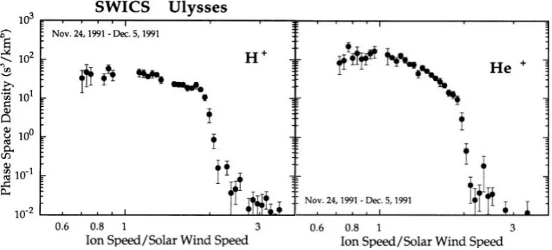
Figure 6: 1D velocity spectrum of pickup protons and He+ observed by the SWICS instrument in the spacecraft frame [Gloeckler et al., 1993].

are not visible, and it becomes very difficult to resolve these sub-processes [Drews et al., 2015].

Immediately after ionization the PUI VDF is assumed to resemble a torus in velocity space, as seen in Figure 5. The torus is rotationally symmetric about the magnetic field with a inclination subsequently defined by the local magnetic field direction [Drews et al., 2015]. If the magnetic field is perpendicular to the solar wind, which is assumed to be radial, the PUI velocity ranges from 0km/s to 2*Vsw, creating a VDF that falls off at 2vsw. If the magnetic field points at small angles relative to the SW, the PUIs will be

gyrate only minimally, causing the VDF to have strong 1st order anisotropy in the SW frame [Saul et al., 2004]. This means that particles injected closer to the Sun will have higher parallel velocity components and smaller ring distributions in velocity space due to the Parker spiral of the interplanetary magnetic field being more radial.

2.4 Transport Effects on the VDF

(17)

Figure 7: Velocity space diagrams depicting the He+ torus distribution under pitch angle scattering (1), adiabatic cooling (2) and rapid changes of the magnetic field vector (3) [Drews et al., 2015]

scattering and for different IMF directions. As the solar wind convects outward, it carries the magnetic field with it, causing the magnetic field and PUI population to expand as the solar wind expands. This effect results in adiabatic cooling of the SW, a decrease in SW density and a decrease in magnetic field strength. For slow variations of B, particles obey the first adiabatic invariant µ:

µ= v

2

⊥

2|B| (5)

Thus a slow decrease in the magnetic field strength will cause a corresponding decrease in

v⊥, shown in Figure 7(2), shrinking the torus, but still retaining its original orientation.

Under these effects, PUIs fill the phase space within the shell, and the cutoff is less pronounced. These processes act over time, so measuring particles that were produced locally will have had less of an effect.

(18)

Figure 8: Velocity vector addition of PUIs with different initial radial velocities and the effect on their 1d PUI VDF. Case (1) shows an injection speed of zero in the inertial frame and a max velocity of twice the solar wind speed. Case (2) shows the effect of a positive injection speed, seen upwind where the interstellar neutral flow is ramming into the SW. Case (3) shows a negative injection speed, seen down wind where the interstellar neutral flow is running away from the SW, the max PUI velocity is lower than 2vsw [Taut,

2018]

2.5 Longitudinal Variation of the Neutral Injection velocity

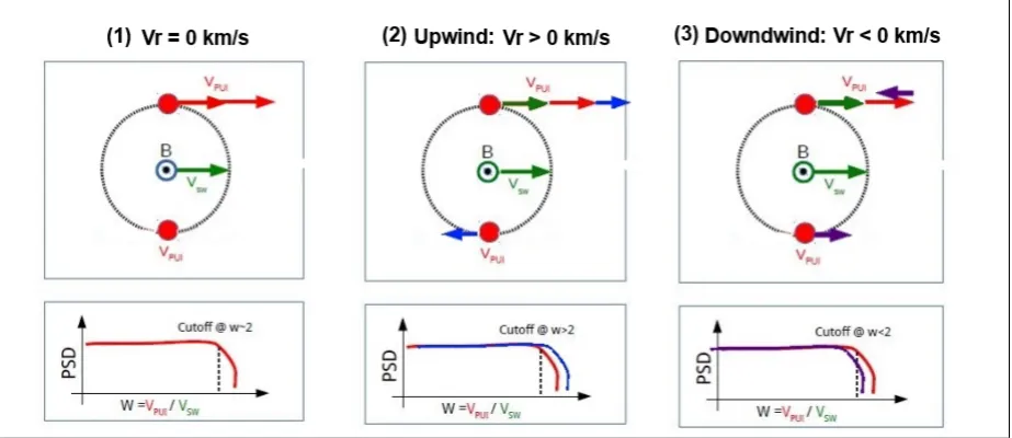
In the past, PUI distributions have typically been evaluated with the assumption that the velocity of their interstellar neutral source is negligible(∼ 25km/s at ∞, compared to an average SW velocity of∼400km/s). However, in this study the injection speed of the PUIs is very important [Moebius et al., 2015b]. Although the interstellar neutrals start from a speed of ∼ 25km/s, as they get closer to the Sun they accelerate into the Sun’s gravitational well, increasing the speed of the neutrals to ∼ 50km/s at 1AU and bending their trajectories (Figure 4). This effect was first discovered in [Moebius et al., 1999] using He+ observation taken with SOHO CELIAS CTOF. In the framework of just the Lorentz force transport, the motion of the PUI depends just on the magnetic field direction, strength and the relative velocities of the ions to the solar wind.

The PUI velocity is typically represented in terms of the PUI speed normalized to the solar wind speed; w=vP U I/vsw. Resulting in a cutoff of approximately wcutof f = 2. The

(19)

Figure 9: Top: He+ PUI cutoff identified in 1deg longitudinal bins, the light blue line overlay is a model fitting of the neutral inflow speed, the blue line designates the upwind flow direction determined through the fit. Bottom: He+ PUI VDF observed by PLASTIC on STEREO-A, the white line designates the inflow direction determined through fitting [Taut et al., 2017].

gyrate around the field with a resultantwcutof f = 2. Upwind, shown in Figure 8 (2), the

SW and the interstellar wind are ramming into one another, this results in an increased relative speed between the neutral He and the SW and a cutoff velocity of wcutof f >2.

Downwind, shown in Figure 8 (3), the opposite effect takes place, the interstellar wind is flowing in the same direction as the solar wind causing a reduction in their relative speed, and a cutoff velocity of wcutof f <2.

Transforming into the solar wind frame alleviates the need to worry about the motional electric field, the orientation of the IMF, and scattering due to Alfven waves; w_{cutof f}0 = (~vP U I −~vsw)/vsw, resulting in an approximate cutoff value of 1. Ignoring the motion of

(20)

radial velocity of the injected neutral (vr) as:

w0_{cutof f} = vsw−vr

vsw

(6)

Upwind, the radial injection speed is negative, resulting in the 1D VDF falling off w >1. Downwind, the injection speed is positive, yielding cutoff value at lower velocities. This effect is continuous as STEREO-A orbits the Sun, and the result is an approximately sinusoidal curve that is symmetric about the ISM flow direction. This effect can be seen in the phase space density plot in Figure 9 (bottom). The cutoff velocity is identified for each 1deg bin, resulting in a functional relationship between vrcutof f and the ecliptic

longitude, seen in Figure 9 (top). In [Moebius et al., 2015b] an analytical model of this effect of the radial neutral speed is derived,

ν_r2 = 2 +ν_ISN2 ∞−(1−cosλ)−[νISN2 ∞sin2λ+{νISN∞

×sin|λ|

q

ν2

ISN∞sin2λ+ 4(1−cosλ)}]/2

(7)

where the neutral particle speed at the observer is given by νr = _vvr

E and the neutral

particle speed at infinity is given by νISN∞ = vISN∞_v

E . These values are normalized to

vE =

q GMs

RE , where G is the gravitational constant, Ms is the solar mass, and RE is

the Sun-Earth distance (1AU). The value λ contains both the interstellar flow longitude and the observed flow longitude: λ = λobs −λinf low. This model can be fit directly to

the measured relationship between vr and λobs, by varying the flow velocity and inflow

direction in a least-square fit. Figure 9 (Top) shows the result of this fit as a light blue line overlaid on the measurements. This results in an upwind flow direction of

λinf low = 255.5±.5◦, and is shown as a vertical blue line in Figure 9. A model free

method of inflow determination is used in [Moebius et al., 2015b], where the authors instead performed a mirror correlation on the vrcutof f(λobs), resulting in a statistically

(21)

3 STEREO PLASTIC

Here we provide some background on PLASTIC, an instrument developed at the Uni-versity of New Hampshire, which is aboard the STEREO spacecraft. This instrument provides PUI measurements in the solar wind frame and solar wind parameter measure-ments that we here use for analysis.

3.1 Mission and Spacecraft Overview

The Solar TErrestrial RElations Observatory (STEREO), launched October 26, 2006, is comprised of two semi-identical, Sun orbiting spacecraft that are drifting apart by 45◦ a year in solar longitude [Galvin et al., 2008]. The primary purpose of the STEREO mission is to study the origin and evolution of Coronal Mass Ejections (CMEs) with a combination of imaging from two vantage points and in-situ measurements of the plasma, energetic particles, magnetic field, and electromagnetic waves [Galvin et al., 2008]. The two spacecraft are STEREO-A (AHEAD), which orbits at a slightly smaller radial dis-tance from the Sun, when compared to Earth, and STEREO-B (BEHIND), which orbits at a slightly larger distance. Therefore, the two spacecraft drift away from the Earth’s orbital positionat a rate of ≈22.5◦ per year [Galvin et al., 2008]. The increasing separa-tion of the two spacecraft allows for multi-point observasepara-tion of the solar wind’s magnetic topology, plasma temperature and density, and temporal evolution of CMEs [Kaiser and et al., 2005]. The STEREO science payload consists of 13 instruments, making up four experiment packages: two instruments suites and two single instruments, each with their own primary science goals [Kaiser and et al., 2005]. Figure 10 (a) shows a schematic depicting the placement of the instrument aboard STEREO-B. The experiment packages are known as [Kaiser and et al., 2005]:

• SunEarth Connection Coronal and Heliospheric Investigation (SECCHI)

Suite:

Comprised of 4 Remote sensing instruments, two White Light Coronagraphs, imag-ing in visible light, an Extreme Ultraviolet Imager, and a Heliospheric imager. The purpose of this suite is to study the 3D evolution of the structure of CMEs from the surface of the Sun to their impact at Earth [Howard et al. 2007].

• In situ Measurements of PArticles and CME Transients (IMPACT) Suite

(22)

(a) (b)

Figure 10: (a) Basic schematic showing the primary instruments aboard STEREO. PLAS-TIC can be seen mounted on the Sun-facing side of the spacecraft [Kaiser and et al., 2005]. (b) Photograph of the PLASTIC sensor taken before mounting. The Sun-facing side of the 360deg entrance system is shown equipped with a small channel aperture to reduce SW flux [Galvin et al., 2008].

interplanetary magnetic field, energetic electrons and ions, and thermal and super-thermal electrons [Luhmann et al. 2007]

• STEREO/WAVES (S/WAVES):

Three orthogonal monopole antenna functioning as an interplanetary radio burst tracker to observe the onset and evolution of radio disturbances between the Sun and Earth [Bougeret et al. 2007].

• PLAsma and SupraThermal Ion Composition (PLASTIC):

Developed to study in situ, the properties of SW protons, the composition and prop-erties of minor solar wind ions, and the distribution of pickup ions and suprathermal ions in interplanetary space [Galvin et al., 2008]

(23)

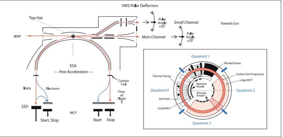
Figure 11: Schematic showing a cross section of PLASTIC’s top hat electrostatic analyzer (ESA) and time of flight system (TOF) (left). The detector plane (right), is sub-divided into 4 quadrants, with quadrant 0 facing the solar wind. Quadrant 0 and 1 contain Solid State Detectors(SSDs) and microchannel plates (MCP’s) with resistive anodes to determine the position of particle entry. [Galvin et al., 2008]

3.2 PLASTIC

(24)

Figure 12: a) Diagram depicting the torus injection (green) on a shell in velocity space. b) Cross section of the spherical shell and torus in the (x,y) plane, showing the torus in the spacecraft frame (green) and in the SW frame (grey) [Taut et al., 2017].

largest azimuthal FOV and as such has the largest geometrical factor, but lower angular resolution than the Solar Wind Sector [Galvin et al., 2008]. After passing the entrance system, particles leave the ESA, undergo post-acceleration and enter the Time-of-Flight chamber (TOF). As implied by its name, the TOF measures the flight time of the par-ticle over a known distance, when coupled with the post acceleration, determines the particle’s Energy per Mass (E/M). Finally, the particle hits a Solid State Detector (SSD) that measures the total energy. A stop signal is provided by a microchannel plate (MCP) that is constructed using a series of resistive anodes to resolve the incoming direction in azimuth. Figure 11, left, shows a schematic cross section of the entrance system, TOF detector, and electrostatic analyzer. On the right is an illustration of the sensor system with the quadrants labeled (quadrant 0 resolves azimuth angle in the SW sector).

The PLASTIC solar wind sector provides the unique capability to measure the incident angle of ions in both polarθ, and azimuthal directions α[Drews et al., 2015]. Azimuthal detection is achieved through a chain of resistive anodes behind the MCP, capable of resolving 32 different angles, with a total FOV of α±22.5◦, resulting in an angular bin width of ∆α = 1.4◦. The polar detection is achieved through an electrostatic deflection system, shown in Figure 11, left, attached to the top of the ESA [Taut, 2018]. This deflection voltage is stepped incrementally 32 times every 435 ms, resulting in a polar FOV ofθ±20.0◦ and an angular resolution of ∆θ = 1.3◦. Additionally, PLASTIC provides the solar wind proton density (n), the solar wind speedvsw and the proton thermal speed

vth.

(25)

et al. [2010], used to resolve each particle’s E/M, E/Q, E, and incoming azimuth and elevation angle. The particle type is determined through the combination of E/Q and E/M resulting in a clearly defined M/Q = 4 for He+. With the particle type (mass and charge) determined, the incoming particle velocity can simply be calculated from the incoming energy determined with the ESA. For each incident He+, PLASTIC yields a measurement of the PUI velocity (vhe+) and incident angles (α, θ) on a 5 min time

resolution. Traditionally, the PUIs have been measured by representing the PUI velocity measured in the spacecraft framew=vHe+/vsw, i.e. normalized to the solar wind speed.

This measurement is fundamentally variable, as the PUI will have a w value between 0 and 2, for a perpendicular field orientation (Figure 5, left), depending on where they are in their gyro-orbit. Additionally, the max cutoff value is dependent on the magnetic field direction, in the sense that for magnetic field orientations far from perpendicular the max cutoff value is also reduced. In the solar wind frame, the PUIs are injected onto a spherical shell in velocity space with a radius that equals the solar wind speed. Figure 12 (a) shows the PUI torus in the spacecraft frame (green) projected onto a shell in velocity space. Changes in the solar wind velocity will affect the radius of the torus by changing the radius of the shell. Changes in the IMF orientation will also change the radius of the torus by intersecting a different part of the shell. Figure 12 (b) shows a cross section of the shell and torus in the (x,y) plane. One can see that the torus diameter (green) will change its length depending on the field orientation. To account for this, PUI measurements can be considered in the solar wind frame, the equivalent of making the center of the circle the origin. From here, regardless of the IMF orientation, the Torus in the SW frame, seen as a gray line in Figure 12 (b), will always be located at a distance associated with the radius of the shell, or approximately the solar wind speed. Thus the PUI measurements should be expressed in the solar wind frame, by subtracting the solar wind velocity from the He+ measurement using their velocity vectors. The relative velocity of PUIs, w0, with respect to the local solar wind speed is given by [Drews et al., 2012]:

w0 = vecvsw−~vHe+

vsw

=pw2₋₂_∗_w_∗_cos(_α_{) cos(}_θ_{) + 1} ₍₈₎

With the PUIs in the solar wind frame the injection speed is conserved for all IMF orientations [Taut et al., 2017]. Essentially, PLASTIC’s angular resolution is paramount as the transformation into the solar wind frame allows us to integrate over STEREO’s entire FOV. For any IMF orientation, the max cutoff velocity should fall at approximately

(26)

4 PUI VDF Treatment and Data Structure

STEREO PLASTIC provides the unique ability to determine the three-dimensional veloc-ity distribution of He+ at a resolution of 5◦. This allows us to obtain radial cuts through the distribution in a frame that moves with the solar wind [Moebius et al., 2015b]. The center of STEREO PLASTIC’s SW sector constantly points radially at the Sun, with a field of view of ≈ ±20◦ in the ecliptic and out of the ecliptic, restricting PUI measure-ments that include the torus to times when the magnetic field is near perpendicular to the radial direction. Because STEREO orbits near 1AU, where the Parker spiral is at

≈45 deg, this torus configuration is not favored, but still readily accessible. An example of the two dimensional particle distributions, in viewing angle and energy, obtained by STEREO can be seen in Figure 13. Here the torus is shown measured in PLASTIC’s FoV on the right, where the magnetic field is quasi-perpendicular, and out of the FoV on the left, where the magnetic field is at small angles from the solar wind flow direction. When the torus is within the FoV it is clear that the cutoff falls on the shell at the solar wind velocity. Even though the torus is broad in angle around the shell, possibly due to pitch angle scattering, the cutoff remains intact. When the torus is outside of the FoV, PUIs are still observable, but they are heavily processed and have a greatly reduced cutoff.

It follows that measurements must be restricted to times when the torus falls into STEREO’s FoV so that only freshly injected PUIs are observed. This restrictive mask, is constructed using the magnetic field cone angle (β), which is defined as the angle between theB~, and the position vector~r, from the Sun to STEREO. This value is calculated using the IMF angle: θ out of the ecliptic, and the azimuthal angle φ from~r. Both angles in our data set are defined between ±180◦ so care must be taken with the signs.

β = arccos(cos(|φ|) cos(π/2−θ)) (9) The mask is now defined using 70◦ < β <110◦ for the times when the torus falls within PLASTIC’s FOV. A slightly different approach is used in Taut et al. [2017] where times are restricted using the average PUI guiding center motion. A comparative analysis be-tween the two methods has been performed, and they have produced comparable results. Due to the PUI process, the PUI speed is generally measured relative to the local ambient solar wind speed. Transformation of the PUI speed into the solar wind frame, as described in section 3.2, allows the PUI speed at injection to be conserved for any ecliptic longitude or IMF angle, but normalizing the PUI velocity tovsw introduces a fundamental

(27)

Figure 13: Two dimensional VDF as seen by STEREO PLASTIC. Where w is the nor-malized PUI velocity, and φB is the angle from the Sun-spacecraft line (radial) in the

ecliptic. We can see on the left, for φb angles far from 90◦ the torus falls outside

PLAS-TIC’s field of view, and only heavily processed PUIs are observable. On the right the magnetic field is close to 90◦, and the high particle flux of the torus can be seen.

of w0 onvsw, needs to be considered and accounted for or it will add additional error to

the inflow measurement. To eliminate the influence of varying SW speed, the cutoff is considered in terms of just the neutral radial velocity component vr:

vr =vsw∗w0−vsw (10)

The first term in the definition, vsw ∗w0, corresponds to the total PUI velocity in the

solar wind frame. This essentially means that vr is the difference between the measured

(28)

4.1 PUI Cut-off Determination

Ideally, while looking at an energetically homogeneous PUI spectrum, the PUI cutoff would be a sharp well defined structure. Due to a various influences, such as the energy width of the neutral beam, local heating, acceleration processes and the finite resolution of the instrument, the PUI spectra are smoothed and the cutoff is less defined. Therefore, the exact location of the cutoff must be defined in a reproducible way. Here we discuss three methods of defining the PUI cutoff, each with benefits and disadvantages in different situations. A study was performed in Taut et al. [2017], where they measured the inflow direction, employing each of these techniques, and found that they all produce statistically similar accuracy.

4.1.1 Tanh Fitting

The first technique we will discuss involves fitting the drop off of the energy spectra with a hyperbolic tangent function, as described in [Moebius et al., 2015b]. This was originally used out of convenience, but has proved to be a statistically accurate and consistent measure of the cutoff provided there are adequate statistics. Initially, the maximum of the smoothed PUI spectra is identified, the spectra above this energy is taken and fit with the Tanh function using least squares minimization:

c= (1−tanh((v0−vcutof f)∗a))/2 (11)

Where c is the expected count rate, v0 the measured PUI velocity (represented by w0,vr

etc.), a is a scaling factor andvcutof f the inflection point of the Tanh function, taken to

be our cutoff value. The error value for this fitting technique is estimated from the fit confidence of the cutoff value. The result of this fitting can be seen in Figure 14a, where the velocity distribution of PUI measurements integrated over one longitudinal bin can be seen in red, the Tanh fit can be seen in blue, and the cutoff value determined through the fit is seen as a dashed black line.

4.1.2 Cutoff Fitting Using the Average DeModulated VDF

(29)

(a) (b)

(c)

(30)

entire 7 year data set, and performed an interpolation, giving us a continuous function that can be fit using the least squares method. The maximum count rate is identified and the distribution function beyond the max location is made continuous through polynomial interpolation. We then introduce variation parameters for fitting, defining the slope (m), the shift in height associated with the high velocity tail (∆h) and cutoff (∆vr). This gives us a fitting equation for the count ratec(vr), defined using the interpolated average PUI VDF f(vr).

c(vr) =A∗f(m∗vr−∆vr) + ∆h (12)

A sample fit that is a stress test for this method is shown in Figure 14. The PUI VDF has undergone considerable heating, indicated by the overall horizontal shift in the VDF and quantified by the ∆vr value. Additionally, acceleration processes result in a massive high

velocity tail, greatly reducing the steepness of the drop off, and a vertical shift accounting for the large fluxes in the tail. Aside from being stable in such extreme conditions, this method to quantifies the steepness of the cutoff, which can be used as a proxy for the amount of accelerated particles in the tail.

4.1.3 Half Max

The half max technique is fairly self explanatory, and is by far the most rudimentary of the three methods. Essentially this method defines the PUI cutoff as the point in the high energy drop off where the count rate reaches half of its max value. While quite simple, this method has proved to be quite accurate, low cost computationally, and is by far the most stable with low statistics. This means that this technique can be used successfully at the highest time resolution, making it ideal when measuring the PUI cutoff for fast variations of compressions when statistics are low. This method begins by smoothing the VDF with a running average, interpolating the histogram and identifying the maximum in the count rate, in both velocity and count rate magnitude. Using the interpolated VDF, the half maximum height is identified on the side of higher velocity and the velocity at that point is recorded. Figure 14b shows a sample of this routine on a one degree integrated VDF, where the blue line is the smoothed, interpolated VDF and the black line represents the velocity where the half max point it determined. The error of the half max point is estimated by adding, in quadrature, the velocity bin width error to the count rate error superimposed in velocity.

δvr1/2max = q

δv2

(31)

Where δvr1/2max is the cutoff error, δvr is the bin width error, vr1/2max is the cutoff

determined through this routine, f(N) is the interpolated VDF, relating the count rate and the PUI velocity (seen in blue in Figure 14b ), N1/2max is the count rate at the half

the max height, and δN1/2max is the count rate error at the half max position. Since the

half max routine has been found to be the most stable with low statistics it will be the only cutoff identification method used for the rest of this study.

4.2 Removal of Longitudinal Dependence

To reduce the error of the neutral inflow measurement, and to study PUI heating in solar wind compression regions, we will identify solar wind compressions, in several forms, and measure their effect on the PUI cutoff. Due to the fact that PUI count rates are relatively low when using PLASTIC, large integration times must be considered to build a PUI VDF with adequate statistics to confidently measure the cutoff. Compression regions in the solar wind generally happen too fast to effectively build a VDF, thus compression events need to be superimposed in order to identify their effects. But, the PUI cutoff speed is dependent on the longitude of measurement, which varies up to 100 km/s over one orbit. This is a large enough variation that combining PUI counts without accounting for their longitudinal variation will introduce considerable error to a PUI compression parameter study. Therefore, the longitudinal dependence of the PUI cutoff must be removed.

The steps to remove the longitudinal dependence of the cutoff follow the sequence of the analysis to determine the inflow direction. First, for each of the longitudinal bins (in 1◦ increments), the cutoff is obtained from the PUI VDF, using the fitting routine of choice. In this study the half-max routine is used throughout. Second, the deduced cutoff values as a function of longitude are fit to the model for the radial component of the ISN flow velocityvr at Earth’s orbit, eq. 7 [Moebius et al., 2015b]. This provides an

approximate inflow direction (λinf low) and velocity at infinity (vISN∞) for the data set.

Using these parameters in a third step, the PUI data at the highest possible time resolu-tion (10mins) are transformed by subtracting the modeled velocity (vr(calc)(λ)) found by

the fit to equation 7, which results in a “demodulated” radial velocity for the PUI VDF (v_r∗):

v_r∗ =vr−vr(calc) (14)

(32)

(a)

(b)

Figure 15: The two dimensional VDFs integrated in longitude over the 7 yr data set in STEREO’s vr frame, with and without longitudinal dependence. On the top in Figure

(a) the longitudinal dependence is intact and increased cutoff speed upwind around the 250deg mark can be seen. On the bottom, in Figure (b) the longitudinal dependence of the data set is removed, and the cutoff position lies approximately at vr = 0 for all

(33)

study is to analyze specifically the effect of the solar wind variations on the PUI cutoff, the PUI measurements are normalized again to the solar wind speed. This results in a demodulated data set as a function of the dimensionless velocityw∗, which allows a direct comparison with a nominal PUI VDF independent of the solar wind speed value.

w∗=v_r∗/vsw (15)

The rest of this analysis will be performed using thew∗ parameter. Combining the frame transformations, normalization and removal of the ISN flow pattern, w∗ is expressed in terms of the measured PUI speed, vP U I, the solar wind velocity, vsw, ecliptic and

latitudinal direction of the PUI velocity vector (described in section 3.2), α and θ, and the radial cutoff velocity as a function of ecliptic longitude, vr(calc)(φ):

w∗ =

r

vpui

vsw

2

−2vpui

vsw

cosαcosθ+ 1− vr(calc)(φ) vsw

−1 (16)

(34)

4.3 Data Structure

Preprocessing of raw STEREO-A PLASTIC data has been performed at the University of Kiel, Gemany to consolidate the measurements to a workable format. Pulse height analysis is used in [Drews et al., 2010] to identify ion type and to measure the PUI ve-locity vector. These individual PUI velocities are transformed into the solar wind frame, and SW parameters, measured by PLASTIC and IMPACT, have been consolidated and averaged to meet PUI measurement cadence. IMF direction measurements, in eleva-tion and azimuth, have been used to calculate the IMF cone angle, and PUI velocity measurements have been transformed and normalized to w∗. Finally, all individual PUI counts are binned in w∗ to produce an easily manipulatable VDF for every measurement period. This results in a consolidated data set comprised of averaged SW parameter measurements and He+ VDFs (in w∗) determined at a 10min time resolution, spanning STEREO-A’s operation from 2007-2013. Additional years are available to add to the con-solidated data set, and are undergoing preprocessing. Each 10 min measurement period contains the following:

• t: Time (in days from 2007)

• φ: Spacecraft longitude (in Ecliptic longitude defined from the Sun-Earth line at the spring equinox)

• vSW(km/s): solar wind speed

• n(1/cm3_{): solar wind number density}

• |B|(nT): Magnetic field strength

• β: Magnetic field cone angel (section 4)

• PUI phase space density measured in w∗, binned in 75 sectors in the range [−1< w∗ < .74]

(35)

5 PUI Cutoff in Variable Local and Global SW

Con-ditions

The solar wind can undergo considerable changes of local speed, composition, density, magnetic field strength, and temperature, that occur on different time scales. On average these fluctuations are driven by global structural variations, such as stream interaction regions (SIR), coronal mass ejections (CME), interplanetary shocks, or IMF reconnection events, but more local structures, such as transient interaction regions or turbulence can drive changes on a shorter time scale as well. Fundamentally, we don’t care about the classification of structures when analyzing the effects that these solar wind fluctuations have on PUI VDF. Since the primary goal is to simply remove or correct for these effects, it is important to identify all changes in the SW parameter as obtained aboard STEREO. The analysis begins with an unbiased assessment of parameter dependencies of the PUI cut-off at the highest time resolution (5.1). This technique that has been shown to be effective at identifying systematic trends in the PUI cutoff shift in a previous study [Taut et al., 2017], where the authors analyze the dependence on the magnetic field angle. As a next step, the study moves on to generic compression structures. In order to analyze the effect of these generally defined compression structures, it is statistically pertinent to identify as many compression regions as possible, whether they are considered co-rotating interaction regions or transient interaction regions. These events are characterized and identified automatically with a selection routine, allowing for similar compressions to be integrated in a superposed epoch analysis, to find a parameter dependence between the PUI cut-off and the compression strength (5.2). Finally, the most extreme compressions are considered. With shock fronts identified separately, and used as the epoch, solar wind parameters and PUI counts are superimposed according to their shock propagation direction (5.3). This results in a maximum PUI cut-off at the shock front passing.

5.1 Local Fluctuations of SW Parameters

(36)

Figure 16: PUI VDF as a function of w∗ for different values of local velocity gradients. The VDF for the largest local gradients (red) is shifted to larger w∗, while for gradients close to zero (blue, purple) the VDF has the lowest cut-off value.

resolution. The 7 year data set is sorted in one of the SW parameters and divided into sections with increasing parameter value. In each of the sections, the SW parameter is averaged and the PUI counts are integrated, giving a single 1D VDF. The cutoff value for each of these spectra is then determined using one of the Half-Max routine. This analysis results in a measurement of the PUI cutoff as a function of a single SW parameter and is used repeatedly to de-construct systematic trends in the cutoff shift due to the local solar wind conditions. Being that the solar wind is an incredibly dynamic environment, one must recognize that solar wind parameters may be linked in some way, and thus one must be careful when trying to determine the effect of a single parameter. Toward the goal to improve the ISN flow measurement, simply identifying criteria in solar wind mea-surements that result in a shifted PUI cutoff results in a filter to remove highly perturbed PUI times.

The derived-parameters, dvsw/dt an dB/dt, are first be calculated using the

(37)

(a) (b)

(c) (d)

(e)

(38)

such that at a specific time increment n, the solar wind speed and field gradients are:

dvn_sw/dt= v

n+1

sw −vnsw−1

2∆t (17)

and

dBn/dt= B

n+1₋_Bn−1

2∆t (18)

B is the field strength, vsw is the magnitude of the solar wind speed and ∆t is the time

step associated with the time resolution of our data set (for this operation: 10 min). The PUI counts are binned for all five parameters. Each list is sectioned into 20 bins of the parameter of interest, such that there are similar statistics in each parameter range. This results in different bin widths in parameter space, as there are fundamentally lower statistics for the largest and smallest values of each parameter. In each range, the parameter is averaged, and the PUI counts are accumulated. This results in 20 PUI VDF’s, each with an associated parameter average. As an example how the PUI PSD varies with interplanetary parameters, Figure 15 shows five of these PUI VDFs sorted in ranges in dvsw/dt. Each of the PUI VDF’s are normalized to the max count rate, and

the cutoff is identified using the half max routine. Figure 17, shows w∗cutof f binned in

20 ranges as a function of d|B|/dt (17c), dvsw/dt (17d), |B| (17a),n(17e) and vsw (17b).

In Figure 16 the most negative dvsw/dtvalue, seen in red, has a visible shift to higher

w∗ values, and the lowest magnitude dvsw/dt, seen in purple, yields the lowest cutoff

value. This essentially means that for decreasing dvsw/dt, where one would expect a

cooling, the PUI’s are seeing a heating. Additionally, for a positive dvsw/dt of smaller

magnitude (yellow), the VDF exhibits a relatively smaller positive shift. This observation is consistent with the dvsw/dt parameter dependence in Figure 17 (b), which shows a

clear positive w_{cutof f}∗ shift for both positive and negative dvsw/dt. A similar response is

visible in Figure 17 (a) where w∗ also shows a positive shift for large gradients in |B|. The strongest linear trend is associated with |B| (c), where w∗_{cutof f} also drops below its average of .025 for small values of |B|. The solar wind density (d), seems to be a poor indicator of PUI heating. With the exception of very high densities, no trend is observed. The largest range between the max and min w∗_{cutof f} is found for the solar wind velocity (e), with a minimum near 400km/s, which is close to the most frequent value for vsw.

5.1.1 Parameter Coupling

(39)

(a) PUI cutoff as a function of field strength for different ranges of sw velocity fluctuations.

(b) Slope of the w∗_{cutof f} and |B|correlation as a function of SW

velocity gradient.

Figure 18: (a) Linear relationships between the PUI cutoff and B field strength in four different ranges ofdvsw/dt(b) Slopes of the cutoff-field strength correlations as a function

(40)

Therefore, similar trends of PUI cutoff with SW velocity and field strength gradients are likely connected with natural coupling between the two parameters. For the SW velocity and field strength gradients this is a fairly intuitive result for quasi-perpendicular IMF orientations that we are restricted to measure. If we measure an increase in the SW velocity, then it follows geometrically that the SW parcel being measured is being com-pressed, as the SW compresses the magnetic field strength in the packet increases because the field lines are being brought closer together. For this reason, these trends cannot be taken at face value and must be further dissected.

Therefore, we will be looking at the relationship between the PUI cutoff, the magnetic field strength and the solar wind velocity fluctuations in combination next. To perform this task, the data is initially as described above to identify cutoff dependence on the velocity fluctuations. The time series ofdvsw/dt, |B|and PUI counts in w∗ are all sorted

in increasingdvsw/dt. Each of these variables are then broken into 14 sections of similar

statistics, according to dvsw/dt, and dvsw/dt in each range is averaged. This results in

lists of |B|and PUI w∗ counts associated with the averagedvsw/dt values. Each of these

sub-lists are sorted according to |B|, and broken up into 10 ranges of field strength. For each of the ranges of this sub-list, |B| is averaged, the PUI counts are accumulated into a single VDF which is normalized, and a cutoff value is identified using the half max routine. This results in a relationship between |B| and w∗_{cutof f}, that changes for each

dvsw/dt. The slope of each of these linear trends is found by fitting a linear function

through least squares minimization. Four of these sample dependencies, between w∗_{cutof f}

and |B|, in ranges of dvsw/dt can be seen in Figure 18 (a). The relationship between

the slope of the cutoff-field strength correlation (dw∗_{cutof f}/d|B|) and dvsw/dt is shown in

Figure 18 (b).

An approximately linear trend is identified between the PUI cutoff and |B| in Figure 17 (c). While Figure 18 (a) shows that a linear trend between w_{cutof f}∗ and |B| for any

dvsw/dt, the slope of the correlation is largely dependent on the magnitude of the velocity

fluctuations. In the blue trend (top left) of Figure 18 (a), there are large negative velocity gradients which result in a cutoff shift of ¯w_{cutof f}∗ =.05 on average. This value is consistent with 17 (d), but when the PUI are sorted for |B|, w∗_{cutof f} shows a range of±.06. This is juxtaposed against the red trend (bottom left), where the magnitude of the SW velocity fluctuations are at a minimum, the trend is essentially flat and the cutoff has a range of ∆w_{cutof f}∗ ≈ .01. This relationship between dw_{cutof f}∗ /d|B| and dvsw/dt seems to be

(41)

Figure 19: Schematic view of a SIR in the ecliptic plane, showing the sequence of com-pression and rarefaction regions. Red indicates the approximate region of the compressed slow wind, purple, the compressed fast wind and blue, the rarefaction region. The black arc indicates STEREO’s trajectory through the SIR. Radial arrows indicate the local solar wind speed. The two large arrows that emerge from the stream interface indicate the compression region expansion into the slow and fast wind. Figure adapted from Pizzo [1978].

velocity gradient. The effect of the coupled negative and positive gradients on the PUI cutoff has not yet been identified, but some information deconstructing the effect of these gradients will be revisited in section 6. after we evaluated the variation of the cut-off shift across identified compression regions and as a function of their strength in the next section.

5.2 Large Scale Compression Regions in the Solar Wind

(42)

compression region evolves, matter piles up at the interface between the two plasmas, separating the high density compressed slow wind (seen in red) and the relatively low density compressed fast wind (seen in purple) [Gosling and Pizzo, 1999]. This pile up, known as the stream interface, is characterized by a large peak in density and increase in proton temperature [Gosling and Pizzo, 1999]. The density maximum is often defined as the stream interface, and we will follow this definition here. Figure 20, shows a sample sequence of three compressions in the SW velocity, number density and magnetic field strength. The sequence of a fast wind and trailing slow wind creates the rarefaction region (seen in blue) where the velocity and pressure decrease and the plasma is cooled. To evaluate the effect that these large compression structures have on the PUI VDF with sufficient counting statistics, we perform a superposed epoch analysis across all compression regions identified in the STEREO data between 2007 and 2013. This analysis is explained in the following.

5.2.1 Compression Region Identification

The process of identifying these compression regions utilizes the SW number density and velocity. SW measurements, which are synchronized with our PUI data sets are measured in 10 min increments. This high time resolution results in substantial local fluctuations that must be removed to see more global structures. Density and speed are averaged in 100 min increments using a nearest neighbor running average. The compression regions of interest occur on time scales on the order of 2 days. Thus, 100 mins is still a relatively high resolution. Peaks, which represent the stream interface are identified in the number density by performing a numerical differentiation of the smoothed time series and identifying the zero crossings [?, Gosling et al., 1996] After the peak finding routine is performed, the most prominent peaks in the number density are selected (top 20%, which are deemed ”large compressions).

(43)

(44)

The compressed fast wind is defined from the stream interface up to the point where the sw velocity stops increasing. The peak region spans between the compressed fast wind and the rarefaction, where vsw is approximately constant. Finally, the rarefaction

region begins when the SW velocity starts to decrease, and continues as long as there is a negative slope. The result of this identification scheme can be seen for a 20 day span in Figure 20.

Here three compression regions are identified, with each section highlighted, red for the compressed slow wind, purple for the compressed fast wind, white for the peak region, and blue for rarefaction region. The red line overplotted on the vsw measurements and

the blue line on the density measurements represent the smoothed time-series used in the peak finding routines. The three compression regions vary in a number of ways. The first compression is rather large, with a solar wind velocity increase of ≈ 300km/s, a peak density value of nearly 50 1/cm3, and a large magnetic field peak. This compression is followed by a long rarefaction region, spanning nearly 5 days, where the density and magnetic field strength are low and calm. The second compression, is much smaller, and is not really considered a SIR at all. While there exists a substantial build up in density, there is only a small increase in the solar wind velocity, and the magnetic field does not return to pre-compression levels in the rarefaction. The third compression, is of comparable magnitude to the first, but instead of a long drawn-out rarefaction region, a second parcel of fast wind arrives.

The compression regions are classified using four different identifiers, the relative change in solar wind velocity (vsw2/vsw1), wherevsw2 is the solar wind velocity at the end

of the compressed fast wind, and vsw1 is the minimum solar wind velocity at the start of

the compressed slow wind. The compression region steepness (∆v/∆t(km/s2_{)) (which is}

(45)

to see underlying trends. We construct an average time series that shows the evolution of the solar wind parameters across the SPE compression region. The start and end times of the slow compressed wind, the fast compressed wind, the peak region, and the rarefaction region (the limits of the colored regions in Figure 20) are used as time stamps for the SPE analysis. Then we stretch or compress the sections of each event in time so that they are all compiled on a similar time scale, referred to as the SPE time. The matching of the times is achieved through performing a running average on the SW parameters of each compression and through binning the PUIs, such that each compression has the same relative time resolution. These time series for each compression are averaged to create the SPE compression, with the end of the compressed fast wind as the epoch. We have chosenvsw, n,|B|,the PUI count rate, and |dvsw|/dtas our SPE SW parameters. Section

5.1 has shown that the PUI cutoff varies substantially with vsw, n,|B|, and |dvsw|/dt,

thus evaluating these parameters across the SPE compression should provide additional insight. Additionally, the PUI count rate will provide insight into the compression effect on the PUI population. The result of this routine, after averaging the largest 20% (based on the steepest SW velocity increase) compressions can be seen in Figure 21.

(46)

Figure 21: Average temporal evolution across the superposition of compression regions, shown here for, SW velocity, density, magnetic field strength, PUI count rate, and mag-nitude of the local solar wind velocity gradient (from section 5.1). Shown is the result from a superposed epoch analysis of 100 compressions selected for large total increases in solar wind velocity. The compression region (blue & purple) shows increasing vsw, peaks

(47)

Figure 22: PUI cutoff (top) and 2D count rate density (bottom) evolution across the SPE SIR event. The max PUI cutoff comes at the end of the compressed fast wind, and drops off substantially going into the rarefaction region. The beginning of the rarefaction region still yields substantially shifted cutoff values.

5.2.2 Evolution of PUI VDF across the SPE Compression

The same SPE averaging across the compression region is also performed on the PUI measurements to see how the PUI VDF and cutoff evolve as a function of time from the end of the compressed fast wind, shown in Figure 22 (bottom). The cutoff in each of the bins in SPE time is now identified using the half max routine, which yields a time-series of w∗_{cutof f} across the SPE compression that can be seen in Figure 22 (top). Evidently, more PUI counts will be accumulated in longer compressions. Which means that they will have a larger effect on the PUI SPE time series.

(48)

Figure 23: PUI VDF as a function of w∗ for four different sample of compressed fast wind, compression strength (∆vsw/∆t) is shown for each distribution in the top right

corner. At the highest compression strength (black), the VDF shows a substantial shift to higher w∗ values and a more substantial high velocity tail.

its peak. The cutoff remains elevated through the peak SW velocity into the rarefaction region, where it bottoms out toward the end, slightly below the average cutoff. Figure 21 also shows that large values of dvsw/dt exist in the peak region and persist into the

rarefaction region. The VDF evolution, seen in Figure 22, shows a visible shift to higher

w∗ in the compressed fast wind and rarefaction region, but an apparent broadening in the compressed slow wind. Additionally, there is an increased flux of high velocity tail particles starting in the compressed slow wind and continuing into the very beginning of the rarefaction region.

5.2.3 Compression Region Parameter Dependence

With the compression regions identified and characterized, the next step is to perform a parameter dependence study, similar to the one performed on the local fluctuations. Each compression region contains a compressed slow wind, compressed fast wind and rarefaction region, that are characterized by the average steepness of the solar wind speed gradient across the region. For each of these regions, the PUI counts are accu-mulated into separate VDFs. This results in lists of compression/rarefaction strengths, and the corresponding VDFs, which are sorted in increasing ∆vsw/∆t and sectioned into

(49)

(a) (b)

Figure 24: (a) PUI cutoff shift as a function of the compression strength in the compressed fast (purple) and compressed slow (red) wind. (b) The PUI cutoff shift as a function of the rarefaction region ∆vsw/∆t. The compressed slow wind, fast wind and rarefaction

regions all seem to show a correlation with|∆vsw/∆t|

parameter study) is the average gradient over the region, calculated using the smoothed

vsw. A sample of four of these VDFs are seen in Figure 23, where a large ∆vsw/∆t

(green) results in a substantial shift to higher w∗. The VDF’s show that for the steepest compressions ∆vsw/∆t = 2.9 there exists a substantial bulk heating of the PUIs. The

separation here is visibly more prominent when compared to the VDF separation of the high time resolution dvsw/dt seen in Figure 16. When compared to the less substantial

compression regions the VDF is shifted to higher w∗ without any flattening that is seen in the local fluctuations.

The cutoff values are plotted as a function of the average ∆vsw/∆tin Figure 24, where

(a) shows the w_{cutof f}∗ dependence on ∆vsw/∆t in the rarefaction region, and (b) shows

the w_{cutof f}∗ dependence in the compressed fast (purple) and slow (red) wind. The cutoff shifts drastically for large compressions and appears to be linearly related to the slope of the compression. In the second plot in Figure 24, the cutoff in the rarefaction region, sorted and accumulated for the rarefaction gradient strength (∆vsw/∆t), appears to be

increasing the steeper decline of the rarefaction region.

(50)

(a) (b)

Figure 25: The PUI cutoff in the rarefaction region, in the time immediately following the compression (a), and in the tail end of the rarefaction (b), revealing a more substan-tial negative correlation between the cooling strength and the cutoff in the top of the rarefaction region than in the tail.

through the rarefaction region, where the PUI counts are accumulated in the top of the rarefaction region separately from the tail of the rarefaction region (dashed vertical line in figure 21). The resulting cutoff values are shown in Figure 25. In the section of the rarefaction region immediately following the compression peak (a), the cutoff varies lin-early with the compression strength, while in the rarefaction tail (b)) there is almost no trend, but the average cutoff is similar to the one in (a).

5.3 Interplanetary Shocks

(51)

Figure 26: Diagram showing the creation of forward and reverse shocks around the in-teraction region of a compression in a stream inin-teraction region. The Forward shock propagates with the solar wind flow direction into the slow wind and the reverse shock propagates against the solar wind flow direction into the fast wind [Steinberg et al., 2005].

front of a CME if the relative motion between the CME and the preceding solar wind exceeds the magnetic sound speed. Because CMEs are such violent events, they are more likely to meet this criterion compared to an SIR [Kilpua et al., 2015]. Additionally, since the occurrence of CMEs correlates with solar activity, so does the total number of FF shocks [Lindsay et al., 2000]. Because the STEREO data set covers solar minimum around 2009, there are fewer FF shocks in the first half of the data set than in the second. The shock normal of the CME-driven shocks on average points more often into the radial direction, while SIRs have a broader distribution of shock normals [Lindsay et al., 2000]. Coupled with the fact that STEREO’s FoV is limited to quasi-perpendicular field directions, FF shocks, associated with CMEs, will be statistically favored when measuring PUIs in shock regions.

(52)

stream interaction regions may be bounded by both a FF shock propagating into the slow wind and a FR shock propagating into the fast wind. The basic structure of this interaction and shock development can be seen in Figure 26. Here, one can see the forward and reverse shocks bounding the interaction region of the SIR at distances beyond 1au. Approximately 24% of SIRs have developed shocks at 1au, and many more of these SIRs will develop shocks as they propagate outward due to the decrease in SW density. [Jian et al., 2006]. Additionally, Figure 26 shows an effective spacecraft trajectory as the interaction region passes over the spacecraft. The effective trajectory means that the spacecraft will pass from the pristine slow wind through the shock front and into the interaction region in a FF shock, and from the interaction region through the shock front and into the pristine fast wind in a FR shock.

As in section 5.2, for compression and rarefaction regions, we superimpose all forward and all reverse shocks so that there is sufficient PUI statistics to determine heating of the torus particles. Creating an SPE time-series for interplanetary shocks is more straight forward than for compression regions, because the shocks only have one relevant structure (the shock front), the times around the shocks can be mapped 1:1. The shock times for STEREO A were taken from IPshocks.com for the entire time of operation of the satellite. With the shock fronts as a reference point, the solar wind parameters 200 mins before and after each shock are considered. The time series for each parameter can then just be averaged point by point with all of the other shocks. The PUI accumulation is similar, for each parameter measurement there is a PUI VDF, so at each measurements in time around the shock front, the PUIs are accumulated, normalized and the cutoff is determined using the half-max routine.

5.3.1 VDF of Fast Forward and Fast Reverse shocks

(53)

Figure 27: Time series of the solar wind parameters, vsw, np and |B| the PUI cutoff

(54)

Figure 28: Time series of the solar wind parameters, vsw, np and|B|the PUI cutoff and

Response of the PUI Distribution To Variable Solar Wind Conditions

University of New Hampshire

University of New Hampshire Scholars' Repository

Response of the PUI Distribution To Variable Solar

Wind Conditions

Jonathan Slade Bower

Response of the Pickup Ion

Distribution to Variable Solar Wind

Conditions

By:

Jonathan

Bower

Contents

1

Introduction

2

Generation and Transport of PUI’s

2.1

PUI Generation and Neutral Sources

2.2

PUI Gyration

2.3

Measurements of the PUI VDF

2.4

Transport Effects on the VDF

2.5

Longitudinal Variation of the Neutral Injection velocity

3

STEREO PLASTIC

3.1

Mission and Spacecraft Overview

3.2

PLASTIC

4

PUI VDF Treatment and Data Structure

4.1

PUI Cut-off Determination

4.2

Removal of Longitudinal Dependence

4.3

Data Structure

5

PUI Cutoff in Variable Local and Global SW

Con-ditions

5.1

Local Fluctuations of SW Parameters

5.2

Large Scale Compression Regions in the Solar Wind

5.3

Interplanetary Shocks

_Bower