Original Research
Modelling the dynamics of CD4+ T cells with and without delay
J. Hussain and R. Lalawmpuii*
Department of Mathematics and Computer Science, Mizoram University, Aizawl 796004, India Received 5 November 2013 | Revised 2 December 2013 | Accepted 5 December 2013
A
BSTRACTAcquired immunodeficiency syndrome (AIDS) is one of the most serious public health problems in the world, which greatly affects the socio-economic growth. Mathematical models can serve as tools for understanding the epidemiology of human immunodeficiency virus (HIV) and AIDS. In this paper, we consider a mathematical model having three compartments. Uninfected and in-fected states are proposed and analysed. It is found that the uninin-fected state is locally stable when the reproduction number R0 < 1 and the infected state is locally stable when R0 ≥ 1 and globally stable when R0 > 1. The model is analysed with and without delay. Numerical simulations are car-ried out to illustrate the results.
Key words: AIDS; HIV; CD4+ T cells; stability; delay.
Corresponding author: Lalawmpuii Phone: +91-0389-2330874
E-mail: [email protected]
I
NTRODUCTIONAIDS is medically devastating to its victims, and causes financial and emotional havoc on the infected person and his/her relatives. The pur-pose of this paper is to model and understand the behaviour of the causative agent of AIDS that is HIV. HIV targets, among others, the CD4+ T lymphocytes, which are the most abun-dant white blood cells of the immune system (referred to as helper T-cells or CD4+ T cells). Helper T-cells play a key role in the process of gaining immunity to specific pathogens; in fact, if one’s helper T-cells are destroyed, the entire
specific immune response fails. HIV kills the very cells that are required by our bodies to de-fend us from pathogens, including HIV itself.1
Several models have been developed in an attempt to understand the dynamics of infec-tious diseases.2-13 In particular, Murray et. al.14
determined the viral level after the initial peak, by the rate of reactivation of memory cells. Perelson et. al.15 observed that the model exhibits
many of the symptoms of AIDS seen clinically; the long latency period, low levels of free virus in the body, and the depletion of CD4+ T-cells. They defined the model by considering four compartments: uninfected cells, latently infected cells, actively infected cells and free virus. They described the dynamics of these populations by a system of four ordinary differential equations.
www.sciencevision.org
192 Science Vision © 2013 MAS. All rights reserved
Mathematical analysis of the global dynam-ics of a model of HIV infection has also been studied by many authors.16-18 Elaiw16 has
con-structed Lyapunov functions19 to establish the
global stability of the uninfected and infected steady states.
In this paper, we consider three compart-ments: the uninfected CD4+ T-cells, the infected CD4+ T-cells and the free virus. The existence and stability of the uninfected and infected states are considered. Time-delay model is also pro-posed and analysed, considering the delay be-tween the infection of CD4+ T cell and emission of virus particles on a cellular level.20-23
M
ATHEMATICALM
ODELA basic model to study HIV dynamics can be described by the following equations:
( )
( ) ( ) ( )
dT t
dT t kV t T t
dt
( )
( ) ( ) (t)
dT t
kV t T t T
dt
(2.1)
( )
( ) ( )
dV t
N T t cV t
dt
In the above model, T, I and V are the concentrations of uninfected CD4+ T cells at time t, concentrations of infected cells at time t and concentrations of free virus at time t respectively, λ is the recruitment rate of uninfected T cells, d is the per capita death rate of uninfected cells, k is the rate constant at which uninfected cells are infected by free virus, δ is the per capita death rate of infected cells, N is the total number of virus particles produced by productively infected cells during its lifetime (burst size), c is the clearance rate of virus, kVT gives the mass action and Nδ gives the per capita viral production. Here, τ is the time delay between infection of the CD+T cells to the cells becoming actively infected.
Model without delay
When τ = 0, the model (1)-(3) reduces to the following model
When τ = 0, the model (1)-(3) reduces to the following model
( )
dT t
dT kVT dt
( )
dT t
kVT T
dt
(3.1)
( )
dV t
N T cV dt
The above system has two non-negative steady states,
1 , 0, 0
E d
and E ( ,2 T T V, )
.
2
E
exists when cdkN
. That is, R01, where
0
kN R
cd
, the reproductive ratio, that is, the number of secondary infections in a healthy host caused by a single infected cell.
Stability Analysis
Theorem 1. The non-infected state E1 is locally
asymptotically stable when
0 1
R
Proof. The Jacobian matrix of the system at the
non-infected state
1
E is
1
0 0 0
k d
d k J
d
N c
All eigenvalues of
J
1 have negative real parts. HenceE
1 is locally asymptotically stable.Theorem 2. The infected state
E
2 is locally asymptotically stable when R01.The detailed proof is shown in appendix A.
Lemma 1. The bounded set
( ), * ( ), ( )
3: 0 * ,S T t T t V t R T T V K
d
is positively invariant with respect to the system (3.1).
The proof of the lemma is given in Appendix B.
Theorem 3. The infected steady state
E
2 is globally asymptotically stable when R01. In the bounded set
( ), * ( ), ( )
3: 0 * ,S T t T t V t R T T V K
d
The proof is shown in Appendix C.
Model with Delay
Here we introduce a time delay into the basic model to describe the time between infection of the CD4+ T cells to the cells becoming actively infected. The model is
( )
( ) ( ) ( )
dT t
dT t kV t T t
dt
( )
(
) (
)
(t)
dT t
kV t
T t
T
dt
(5.1)( )
( ) ( )
dV t
N T t cV t
dt
Again we find the uninfected steady state
3
E ( , 0, 0)T and E ( ,4 T T V, ) .
At E ( , 0, 0)3 T , from equation (4), we get
T d
. Thus
3 , 0, 0
E d
is the uninfected steady
state.
At
E ( ,
4T T V
, )
, from equation (3),N T V
c
Putting this value of
V
in equation (2), we obtain T ckN
Again putting N T V
c
in equation (1), we
get T 1 cd kN
Thus
4
1
E c , cd , N T
kN kN c
, that
is, E4 c ,1 cd ,k N dc
kN kN kc
is the
infected steady state.
Theorem 4. Suppose
(i) 0, 0 and 0 (ii)
d
Then the infected steady state
E ( ,
4T T V
, )
of the delay model is asymptotically stable when
0 1
R for all
0.The proof is given in Appendix D.
Numerical Simulations
We choose the following parameters in the model:
With the above values of parameters, the positive equilibrium
E
2exists and it is given by*
2.968, 0.147, 0.094
T T V
Also, with the above values of parameters,
0 1.122 1
R
Hence the condition in theorem 2 is satisfied.
Also, the three inequalities in Theorem 3 are satisfied with C10.1,
C
2
5
,K
5000
.With the above parameters,
1.5790 0, 0.0577 0, 0.9354 0
Hence conditions (i) and (ii) of Theorem 4 are also satisfied.
a)
Behaviour of uninfected cells for different values of k
Behaviour of uninfected cells with respect to time for different values of the rate constant at which uninfected cells are infected by free virus.
1,
d
0.3,
k
0.4,
0.75,
c
0.95,
N
0.8
1, d 0.3, k 0.4, 0.75, c 0.95, N 0.8
194 Science Vision © 2013 MAS. All rights reserved
Figure 1
It is noted here that the density of uninfected cells increases as k decreases. It is also observed that T increases rapidly and gradually reaches a steady state.
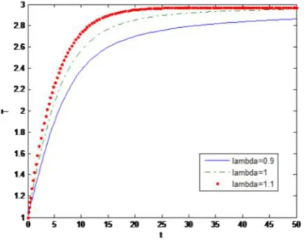
b) Behaviour of uninfected cells for different values of
lambda
Behaviour of uninfected cells with respect to time for different values of the recruitment rate of uninfected T cells.
Figure 2
It is noted here that the density of uninfected cells increases as lambda increases. It is also ob-served that T increases rapidly and then reaches a steady state.
c) Behaviour of infected cells for different values of
lambda
Behaviour of infected cells with respect to time for different values of the rate constant at which uninfected cells are infected by free virus.
Figure 3
It is noted here that the density of infected cells increases as k increases. It is also observed that T* decreases rapidly and then reaches a steady state.
d) Behaviour of free virus for different values of N
Science Vision © 2013 MAS. All rights reserved 195
Figure 4
It is noted here that the density of free virus increases as N increases. It is also observed that the population of free virus decreases rapidly and gradually reaches a steady state.
e) Behaviour of uninfected cells, infected cells and virus
with respect to time with τ = 1
Figure 5
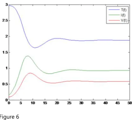
f) Behaviour of uninfected cells, infected cells and virus
with respect to time with τ ≈ 0
Figure 6
From Figure. 5 and Figure. 6, it is seen that in the presence of delay, the population of infected cells and the population of virus increases at a slower rate.
Conclusions
In this paper, we have studied the basic dynamic model of CD4+ T-cells. The model has three differential equations dealing with the interactions between the uninfected cells, infected cells and free virus. A decrease in density of uninfected cells has been observed upon interaction with virus. The density of infection increases with viral interaction. Existence of equilibrium points and the conditions for local and global stability have been obtained. The basic reproduction number
0
R is obtained and it determines the dynamics of
the HIV models. It is seen that the infection is cleared out when R01 whereas the infection persists when
0 1
R . A time delay
i.e. thetime delay between the infection of CD4+T cell and the emission of virus particles on a cellular level, has been incorporated. It is found that the solution of the delay system converges to the disease free equilibria if R01. The infected steady state is asymptotically stable for all
0when
0 1
R .
Appendix A: Proof of Theorem 2
The Jacobian matrix of the system at the infected state E2 is
2
0
0
d
kV
kT
J
kV
kT
N
c
The characteristic equation is
3 2
2 1 0 0
A A A
(1)By using the transformations
1 1
t
T
T
*
2 2
t
T
T
1 1
196 Science Vision © 2013 MAS. All rights reserved
Appendix A: Proof of Theorem 2
The Jacobian matrix of the system at the infected state E2 is
2
0
0
d
kV
kT
J
kV
kT
N
c
The characteristic equation is
3 2
2 1 0 0
A A A
(1)By using the transformations
1 1
t
T
T
*
2 2
t
T
T
1 1
v V V
We linearize the system
.
1
1 .
2 2 2
.
1 1
T
T
T J T
V V
and get
.
1 1 1
.
2 1 2 1
.
2 1
1
T d kV T kTV
T kVT T kTV
N T cV
V
Consider the following positive definite function
2 2 2
1 1 2 2 1
1 2
X T C T C V
Then
i.e.
2 2
2 2 2
21 1 1 2 1 2 1 1 1 2 1 1 2 2 1 2 1 2 1
1 1 1 1 1 1
2 2 2 2 2 2
X dkV T C kVT T C T dkV T kT TV cC V C T C NC kT T V cC V
2 2
2 2 2
21 1 1 2 1 2 1 1 1 2 1 1 2 2 1 2 1 2 1
1 1 1 1 1 1
2 2 2 2 2 2
X dkV T C kVT T C T dkV T kT TV cC V C T C NC kT T V cC V
2 2
2 2 2
21 1 1 2 1 2 1 1 1 2 1 1 2 2 1 2 1 2 1
1 1 1 1 1 1
2 2 2 2 2 2
X dkV T C kVT T C T dkV T kT TV cC V C T C NC kT T V cC V
2 2 2 2 2 2
11 1 12 1 2 22 2 11 1 13 1 1 33 1 22 2 23 2 1 33 1
1 1 1 1 1 1
2 2 2 2 2 2
X A T A T T A T A T A TV A V A T A T V A V
i.e.
where
11
22 1
33 2
12 1
13
23 2 1
A d kV
A c
A cC
A C kV
A kT
A C N C kT
Sufficient conditions for Xto be negative
definite are that the following inequalities hold
2
12 11 22
2
13 11 33
2
23 22 33
A A A
A A A
A A A
The last inequality is satisfied if R01 .
Appendix B: Proof of Lemma 1
Adding the first and the second equations of system (3.1),
. .
* * *
0
T T
dT
T
d TT (since
d
)So both the uninfected and infected T-cell populations are always bounded.
Also from the third equation,
𝑉 =𝑁𝛿𝑇
∗
𝑐
Therefore, 𝑉 ≤ 𝐾, for some 𝐾 ≥ 0. Thus we have a bounded set
3( ), * ( ), ( ) : 0 * ,
S T t T t V t R T T V K
d
that is positively invariant with respect to system (3.1).
Appendix C: Proof of Theorem 3
2 2
2 2 2
21 1 1 2 1 2 1 1 1 2 1 1 2 2 1 2 1 2 1
1 1 1 1 1 1
2 2 2 2 2 2
X dkV T C kVT T C T dkV T kT TV cC V C T C NC kT T V cC V
2 2 2 2 2 2
11 1 12 1 2 22 2 11 1 13 1 1 33 1 22 2 23 2 1 33 1
1 1 1 1 1 1
2 2 2 2 2 2
X A T A T T A T A T A TV A V A T A T V A V
2 2 2 2 2 2
11 1 12 1 2 22 2 11 1 13 1 1 33 1 22 2 23 2 1 33 1
1 1 1 1 1 1
2 2 2 2 2 2
Science Vision © 2013 MAS. All rights reserved 197
Appendix C: Proof of Theorem 3
Let Then i.e.
2 2 * * * *1 11 12 22
2 2
11 13 33
2 2
* * * *
22 23 33
1 1 2 2 1 1 2 2 1 1 2 2
V a T T a T T T T a T T
a T T a T T V V a V V
a T T a T T V V a V V
(2) where 11 1
22 * *
33 2
12 1 *
13
23 2 1 *
2
2
3
a
T T
C kVT
a
T T
a
C c
kV
a
C
T
a
k
kT
a
C N
C
T
1V
will be negative definite if
*
2
* * * 2
1( , , ) ln ln *
2
C
T T
V T T V T T T C T T T V V
T T
* 2* * * 2
1( , , ) ln ln *
2
C
T T
V T T V T T T C T T T V V
T T
2 2* * 1 * *
1 1 * * *
2 2
2
2 2
* * * *
1
2 1 2
* * *
2
1 1
2 2
1 1 2
2 2 3
2
1 1 2
2 2 3
C kVT kV
V T T C T T T T T T
T
TT T T
T T k T T V V C c V V
TT
C kV T kT
T T C N C T T V V C c V V
T T T
2 2* * 1 * *
1 1 * * *
2 2
2
2 2
* * * *
1
2 1 2
* * *
2
1 1
2 2
1 1 2
2 2 3
2
1 1 2
2 2 3
C kVT kV
V T T C T T T T T T
T
TT T T
T T k T T V V C c V V
TT
C kV T kT
T T C N C T T V V C c V V
T T T
2 2* * 1 * *
1 1 * * *
2 2
2
2 2
* * * *
1
2 1 2
* * *
2
1 1
2 2
1 1 2
2 2 3
2
1 1 2
2 2 3
C kVT kV
V T T C T T T T T T
T
TT T T
T T k T T V V C c V V
TT
C kV T kT
T T C N C T T V V C c V V
T T T
2 2* * 1 * *
1 1 * * *
2 2
2
2 2
* * * *
1
2 1 2
* * *
2
1 1
2 2
1 1 2
2 2 3
2
1 1 2
2 2 3
C kVT kV
V T T C T T T T T T
T
TT T T
T T k T T V V C c V V
TT
C kV T kT
T T C N C T T V V C c V V
T T T
2 2* * 1 * *
1 1 * * *
2 2
2
2 2
* * * *
1
2 1 2
* * *
2
1 1
2 2
1 1 2
2 2 3
2
1 1 2
2 2 3
C kVT kV
V T T C T T T T T T
T
TT T T
T T k T T V V C c V V
TT
C kV T kT
T T C N C T T V V C c V V
T T T
2 2* * 1 * *
1 1 * * *
2 2
2
2 2
* * * *
1
2 1 2
* * *
2
1 1
2 2
1 1 2
2 2 3
2
1 1 2
2 2 3
C kVT kV
V T T C T T T T T T
T
TT T T
T T k T T V V C c V V
TT
C kV T kT
T T C N C T T V V C c V V
T T T
122 * *
33 2
12 1 *
13
23 2 1 *
2
2
3
T T
C kVT
a
T T
a
C c
kV
a
C
T
a
k
kT
a
C N
C
T
1V
will be negative definite if2 12 11 22
2 13 11 33
2 23 22 33
a a a
a a a
a a a
The last inequality is satisfied if
0 1
R .
Appendix D: Proof of Theorem 4
At the infected steady state E ( ,4 T T V, ), the
linearized system is given by
1 2
( )
( ) ( )
dY t
J Y t J Y t
dt (3)
where
*
(.) (.), (.), (.) T
Y T T V
The characteristic equation of eqn. (3) is
3 2
2 1 0 1 0 0
A A A B B e
(4)where
2
A
c
d
kV
1
A dkV c c
0
A c
dkV1
B kN T
0
B kdN T
When
0
, all the roots of eqn.(4) havenegative real part and for
0
, it has infinitely many roots. By Rouche’s theorem and the continuity in
, eqn.(4) has roots with positive real parts if and only if it has purely imaginary roots.Taking
( )
i
( ),
0
, as theeigenvalue of eqn.(4), where
( ) and
( )depend on the delay
. Since the infected steady stateE ( ,
4T T V
, )
of the ODE model isstable, it follows that
( )0 when
0
. Bycontinuity, if
0
is sufficiently small, we stillhave
( )0 and E ( ,4 T T V, ) is still stable. If0
( )
0
for certain value 00 so that0
( )
i
is a root of eqn.(4), then the steady state E ( ,4 T T V, ) loses its stability and becomes
unstable when ( ) becomes positive. If such an
0 ( )
does not exist, that is, if the characteristic eqn.(4) does not have purely imaginary roots for all delay, then the steady state E ( ,4 T T V, ) is198 Science Vision © 2013 MAS. All rights reserved
R
EFERENCES1. Perelson AS, Kirschner DE & De Boer R (1993). Dynam-ics of HIV Infection of CD4+ T cells. Math Biosci, 114, 81 -125.
2. Dubey B, Dubey US & Hussain J (2011). Modelling ef-fects of toxicant on uninfected cells, infected cells and immune response in the presence of virus. J Biol Syst, 19, 479-503.
3. Dubey B & Dubey US (2007). A Mathematical model for the effect of toxicant on the immune system. J Biol Syst,
15, 473-493.
4. Ball CL, Gilchrist MA & Coombs D (2007). Modeling within-host evolution of HIV: mutation, competition and strain replacement. Bull Math Biol, 69, 2361-2385. 5. Marchuk GI (1983). Mathematical models in
Immunol-ogy, Optimization Software Inc., Publications division, New York.
6. Marchuk GI (1997). Mathematical Modelling of Immune Response in Infectious Disease, Springer.
7. Wu H, Zhu H, Miao H & Perelson AS (2008). Parameter identifiability and estimation of HIV/AIDS dynamic models. Bull Math Biol, 70, 785-799.
8. Ghosh M, Chandra P, Sinha P & Shukla JB (2006). Mod-elling the spread of bacterial infectious disease with envi-ronmental effect in a logistically growing human popula-tion. Nonlinear Anal Real World Appl, 7, 341-363.
9. May RM & Anderson RM (1987). Transmission dynamics of HIV infection. Nature, 326, 137-142.
10. Duffin RP & Tullis RH (2002). Mathematical models of the complete course of HIV infection and AIDS. J Theor Med, 4, 215-221.
depend on the delay
. Since the infected steady stateE ( ,
4T T V
, )
of the ODE model isstable, it follows that
( )0 when
0
. Bycontinuity, if
0
is sufficiently small, we stillhave
( )0 and E ( ,4 T T V, ) is still stable. If0
( )
0
for certain value 00 so that0
( )
i
is a root of eqn.(4), then the steady state E ( ,4T T V, ) loses its stability and becomes
unstable when ( ) becomes positive. If such an
0 ( )
does not exist, that is, if the characteristic eqn.(4) does not have purely imaginary roots for all delay, then the steady state E ( ,4 T T V, ) isalways stable.
Putting i in eqn.(4), we get
Separating the real and imaginary parts, we get
2
2 0 1 0
A
A B Sin
B Cos
(5)
and
3
1 1 0
A B Cos B Sin
(6)Squaring and adding eqn. (5) and eqn. (6), we obtain
Putting 2
m
in the above equation, we get3 2
0
m
m
m
(7)where
2
1 2
2A A
2 2
1 2 0 2 1
A A A B
2 2
0 0
A B
Eqn. (7) may be written as
3 2
( )
0
h m
m
m
m
Now, ( ) 2
3 2
dh m
m m
dm
Set 2
3
m
2
m
0
(8)Then the roots of eqn. (8) can be expressed as
3 2 2
2 1 0 1 1 0 0 0
i
A
A i
A B i Cos
B i
Sin B Cos
B iSin
3 2 2
2 1 0 1 1 0 0 0
i
A
A i
A B i Cos
B i
Sin B Cos
B iSin
2 3 2
2 2 2 2
2 2 21 2 1 0 2 1 0 0
2A A A 2A A B A B 0
2 3 2
2 2 2 2
2 2 21 2 1 0 2 1 0 0
2A A A 2A A B A B 0
2
1
3 3
z
(9)2
2
3 3
z
(10)If 0, then 2 2
3
, hence z10 and z20. Thus eqn. (8) does not have positive
roots. Since h
0 0, it follows that eqn. (7) has no positive roots. Thus if 0 and 0, then there is no
such thati
is an eigenvalue of the characteristic eqn. (4). Therefore, the real parts of all eigenvalues of eqn. (4) are negative for all delay
0
.11. Dumrongpokaphan T, Lenbury Y, Ouncharoen R & Xu Y (2007). An Intracellular delay- differential equation model of the HIV infection and immune control. Math Model Nat Phenom, 2 75-99.
12. Kindt TJ, Goldsby RA, Osborne BA & Kuby J (2007). Immunology, 6th edition. W.H. Freemam and Company, New York.
13. Hraba T & Dolezal J (1996). A mathematical model and CD4+ lymphocyte dynamics in HIV infection, Emerg Infect Dis, 2, 299-305.
14. Murray JM, Kaufmann G, Kelleher AD & Cooper DA (1998). A model of primary HIV-1 infection. Math Biosci,
154, 57-85.
15. Perelson AS & Nelson PW (1999). Mathematical analysis of HIV-1 dynamics in vivo. SIAM Rev, 41, 3-44.
16. Elaiw AM (2010). Global properties of a class of HIV models. Nonlinear Anal Real World Appl,11, 2253-2263. 17. Wang L & Li MY (2006). Mathematical analysis of the
global dynamics of a model for HIV infection of CD + T cells. Math Biosci,200, 44-57.
18. Leenheer PD & Smith HL (2003). Virus dynamic: A global analysis. SIAM J Appl Math, 63, 1313-1327. 19. LaSalle J & Lefschetz S (1961). Stability by Liapunov’s Direct
Method with Applications. Academic Press, New York, Lon-don.
20. Hertz AVM, Bonhoeffer S, Anderson RM, May RM & Nowak MA (1996). Viral dynamics in vivo: limitations on estimates of intracellular delay and virus decay. Proc Natl Acad Sci USA, 93, 7247-7251.
21. Srivastava PK & Chandra P (2010). Modeling the dynam-ics of HIV and CD4+ T cells during primary infection. Nonlinear Anal Real World Appl, 11, 612-618.
22. Culshaw RV & Ruan S (2007). A delay-differential equa-tion model of HIV infecequa-tion of CD4+ T-cells. Math Biosci,
165, 27-39.