The relationship between inflation and economic grow whit switching model and probability matrix

(1)

The relationship between inflation and economic

grow whit switching model and probability matrix

Zahra Parsaeian and Seyed Yahya Abtahi

*

Department of Economic, Yazd science and Research Branch, Islamic Azad University, Yazd, Iran

Corresponding author:

Seyed Yahya Abtahi

ABSTRACT: The study of the effect of great variables on economic growth has been one of the most important issues of improved countries that have formed the economic decisions. The data of this empirical research include a specific season of the year between 1993 and 2011 that are collected through International Bank website; and the econometrics model used is the Self-Regression Threshold Vector. This model examines the relation between inflation and economic growth in a way that it is organized in the form of two equations: one, the economic growth equation, and two, the inflation equation, and in the two regimes, regime one (the lower inflation from the threshold level), and regime two (the higher inflation from the threshold level). The findings of the study show that the threshold amount of inflation estimated in Iran is 7.71. In regime one of the Gross Domestic Product equation, the coefficient of inflation variable has negative relation with the economic growth in the first and the third interval and positive relation with the economic growth in the second interval. However, the coefficient of inflation variable is only significant in the first interval. This illustrates that when the inflation is lower than the threshold value (regime one), the inflation variable can have a significant effect on the economic growth through one interval. Additionally, the findings of switching model declared that the examination of Probability Transfer Matrix shows the tendency of economy to stay more in a slump position.

Keywords: Matrix shows, Threshold, Regime, Inflation.

INTRODUCTION

Inflation is one of the crucial variables in the economy, as inflation control by the government is one of the basic criteria of effective state to be considered and always one of the slogans is the inflation. Inflation can change distribution of wealth and the widening gap between advantageous the capitalist and prosperous people and when there's accelerated inflation by create uncertainty in relative prices reduce production and investment levels. However, gentle and quiet inflation as a reward for the investor because they have seen an increase in fixed assets, and the investment will lead to increased motivation. So helpful or harmful effects of inflation depends on its size.(2007,Dashtee)

Including macroeconomic objectives of economic topics is achieve high and stable economic growth, lower inflation, full employment and the fair distribution of income in the country. inflation is important economic phenomena and imposes high costs on society. The effects of inflation can be traced to redistribution of income in favor of the property owners and investors and the detriment of employees and workers, increasing instability in the macro economy and thus a shortened of decisions time horizon and long-term investment and other factors.(Peraee and Dadvar.2011)

(2)

268

price stability and inflation can be as one of the most important economic variables have a profound impact on economic growth and GDP.( Fountas at el 2002)

Statement of Problem

Relationship between inflation and economic growth in different countries has always been a discussion topic among economists and is different theoretical and empirical issues in this domain . study of many of these issues shows that can not a definite conclusion about the effect of inflation on economic growth can be achieved and This is for every country depending on the conditions and characteristics. However, in most studies, the conclusion is reached that high levels of inflation is negative and sustainable effects on economic growth. So, in recent years central banks have an increasing emphasis on price stability, and monetary policies have been applied to low and stable inflation , To prevent the imposition of higher inflation, because of the perception that inflation has a significant cost, some of the costs associated with the average inflation rate and another variability associated with uncertainty of inflation.

In response to the question of inflation whether the impact on each country's economic growth, it can be stated that this depends on the economic structure of each country . For this reason, the assessment of a country's economic growth, the effects of inflation on growth as one of the factors that affect the economic growth is important.(Mahmoodi Nia At El 2012)

In recent decades, economists have concluded that moderate levels of inflation can contribute to economic growth. The purpose of this level of inflation is not the price high level , causing uncertainty in the economy and hinder the proper functioning of the economy.Is inflation must get to zero? The low inflation rate can be increased to a positive relationship between inflation and economic growth, but high rates of inflation, there is a negative. relationship between these two variables

Literature

Haider (2010) investigate the effect of inflation as anti-nationalist and money on key economic variables autoregresive approach taken by the immediate impact of the shock and demonstrates that the variable And analysis of variance contribution rate varies due to changes in other variables show repeats shocks. According to the results of the Granger causality and impulse response function, the effect of inflation on the exchange rate, but the exchange rate on inflation is statistically ineffective. As the shock of inflation in 3 courses and increasingly on the exchange rate has affected the long-term equilibrium relationship between variables, Johansen test shows.

Sameti and Karimzade and Nilforooshan (2010)have been Analysis of Business Cycles using variables GDP growth, investment growth and consumption growth over the years (2007-1970). Statistical methods used in this study, a model ARMA (pq) is optimal and also the technique of Granger Causality test for causality between variables are used. The results obtained growth are suggest that the causality between the variables of production, consumption and investment And demand side shocks affecting the business cycle movements in Iran has been impressive.

Kmyjany and Tavakkolian (2012) to analyze and test the asymmetry in the behavior of the central bank's monetary policy with Markov switching model for data seasonally adjusted monetary base, the consumer price index (CPI) and gross domestic product (GDP) to obtain the the rate of money growth and inflation and the output gap over the period 1998-2009 is used. Markov switching model estimation results indicate that the central bank of the boom more attention to deviations of inflation from the inflation target oriented While the slump in economic activity for the central bank to raise the more important.

Kholodlin (2006) to predict the German business cycle turning Markov switching dynamic factor model to simultaneously use two leading indicator (CLI) and simultaneously index (CCI) with the corresponding probability has been taken. The data used in this paper, time series data from 147 German industries along with the titles of the four indicators of expectations, interest rates in the money market of the Frankfurt Stock Exchange and prices of raw materials component (CLI) And the titles of the five leading indicator index of industrial production, new orders in manufacturing, retail and export of goods FOB price components (CCI) have been selected. This enables us to measure and predict the turning points in the business cycle is simultaneously. The results show that the dynamic two-factor Markov switching model to identify and predict the turning point of the recession much more useful than single-factor model is dynamic.

(3)

269

is expected to be approximately 3% as reduced, It is possible for the financial politicians on the eve of keeping inflation below 13 percent for proof of a negative impact on economic growth will be useful.

Mandler(2012) In another study by using the threshold autoregressive is examined Effectiveness of monetary shocks policy on inflation regimes in the United States in the period 2007-1965. And has stated that the effects of monetary policy are different for different inflationary regimes. So in terms of low inflation, inflation tends to reduce the price puzzle and , but in terms of high inflation monetary policy is crucial.

Vinayagathasan(2013) Study to investigate the threshold levels of inflation and how the level of economic growth in Asia using dynamic panel focused on the brink of a recursive process. The results indicate a non-linear relationship between inflation and economic growth in 32 Asian countries over the period 1980 to 2009. The inflation threshold is approximately 43/5%, with a significant percentage detected and indicate when inflation is more than 43/5% harms economic growth, but below the surface there is no impact on economic growth.

Tehranchian At El(2013) Research has focused on testing the stability of inflation in Iran . For this purpose, according to the inflation rate of the time series data (2011-1962), the moving average cumulative fractional regression model is used. The results of this study show that the method of maximum likelihood and maximum likelihood adjusted, build up or difference of the order are 482 / 0d1 = and 483/0 d2 =. So based on the above findings, the inflation persistence hypothesis is not rejected in Iran. Due to the gradual liquidation, the impact of inflationary shocks, it is possible to structural inflation and observe of monetary discipline, the most important recommendations of this study are considered.

MATERIALS AND METHODS

In order to achieve the objectives study and hypotheses testing, and due to the nature of the data must be considered; Check static variables and using time series models for the interpretation and analysis of economic relations between the variables. Using the Phillips Perron unit root tests to examine the Manaei of variables used in the model and have been selected autoregressive econometric model captures the threshold (TVAR) in order to examine the objectives and assumptions described.

The population

In this study, survey data on macroeconomic variables are including economic growth, inflation, GDP, money supply, consumer price index and the price index implicit deflator exchange rates. . The data are quarterly data (2011: 4-1992). It should be noted thl data were collected from the World Bank (WDI).

Research Tools

Given that this study is empirical and application requires the use of empirical data. The data collected in this study is based on a library method. Details of the study based on economic data of period 1992 to 2011 that has been collected from the World Bank or the Central Bank of Iran. All statistical analyzes in this study is performed by using the software package Eviews.

Model Research

Model of study is threshold vector autoregressive (TVAR) and data such as gross domestic product (GDP) as dependent variables and inflation (INF) as independent variables. Equation 1, Equation is (GDPR) and the corresponding equation (INF) each of the variables in the model with three lags is that their results are given in detail in the following chapters. Implicit relationships in Equation 1 and 2 are shown.

GDPR =f (GDPRt-1, GDPRt-2, GDPRt-3, inft-1, inft-2, inft-3) )1(

INF =f (GDPRt-1, GDPRt-2, GDPRt-3, inft-1, inft-2, inft-3)

Statistical Analysis Evaluation of variables

Continuing is discussed the trend of the main variables of the model . The economic variables are shown in Figure 1. This chart is known as the largest economy in the years 1976 and minimal is 1980. This review of varies show damping a lot during the years. In recent years the trend of declining economic growth in 2011 was about zero.

Threshold VAR model

(4)

270

different regression parameters with i = 1, ..., s and p-order regression with j = 1, ..., p is. Thus, a threshold VAR model can be written as follows:

i d t i i , t p j j t j , i i

t

c

A

y

if

r

w

r

y







_



_



 



1

A K × 1 vector of disturbances process with mean zero and variance equal to the . Transfer w variable yt is a vector of variables. The nonlinear multivariable model assumes that p is the same for each variable and state transfer function is similar to the equation.

A threshold VAR 2 Regime be written as follows:











t p t p





t d



t

d t p t p t t

r

w

I

y

A

y

A

c

r

w

I

y

A

y

A

c

y

















     

1 ...

...

, 2 1 1 , 2 2 , 1 1 1 , 1 1

Where I (.) Is an indicator function. An example of a threshold 2R-VAR literature, modeling of growth and the gap between long-term and short-term interest rates in the country is America (Galvav 2002). To predict crack growth only when the value is negative, it helps. This implies that a model with a variable transmission gap, the threshold value is close to zero and the values of a21 the matrices A2, j are statistically equal to zero.

A threshold VAR 3 Regime be written as follows:

















 





3 3,1 1 3,





2



2



.

2 2 1 1 , 2 1 1 , 2 2 1 1 , 1 1 1 , 1 1

1 ...

...

t d t p t p t d t d t p t p t p t p t t

r

w

I

y

A

y

A

c

r

w

I

r

w

I

y

A

y

A

c

r

d

wt

I

y

A

y

A

c

y

























        

A temporary organization that is expected theoretical concepts The gap between long-term and short-term interest rates to future changes in short-term rates over the period to maturity of long-term rates have anticipated. When the relationship between short-term rate and the gap with a 3R-VAR threshold were modeled, Pytaraksy (2008) show that the theory is expected to be positive in the three regimes and the large publication, is established, but the gap between the short-term rate is similar to the regime.

Markov switching model and threshold

In this section, the Markov switching and threshold approaches for modeling of "regime change" is used. Suppose we are interested in modeling a time series of simple like Y_t so that Y_t and contingency Mana is a scalar. In most studies, the model of choice to study a model of order k is autoregressive:

yt= α + ∑ ∅jyt−j+ εt k

j=1

,

That the disruption to normal with zero mean and variance ε_t σ ^ 2 is distributed. Autoregresive a model of order k (Equation 1) model is advantageous as a means to establish facts about the dynamic behavior of the time series used And the expected future trend of a time series is in a good performance.

In many cases, you may be dealing with a series of time-series behavior during different periods vary(In other words, in a time series over a certain period, to be confronted with various regimes).

For example, you may be faced with a model switch as follows:

yt= αSt+ ∑ ∅j,Styt−j+ εt

k

j=1

(5)

271

Except disruption to normal with zero mean and variance ε_t σ_ (S_t) ^ 2 is distributed. In relation, AR (k) values (values) associated S_t discrete state variable which indicates the type of regime S_t is at the time. Suppose the model parameters can easily be changed with time. (This kind of model assumptions simplifying assumptions so-called).

Markov switching and threshold models differ in their assumptions about the state variable S_t. Threshold models assume S_t a function of the variable is defined. S_t identical to herself most of the time lag variables in the models appearing in this state regime change "self-induced" refers. In a model of self-induced threshold N-1 has a defined threshold and S_t is defined as follows:

St= 1 yt−d< τ1,

St= 2_. τ1≤ yt−d< τ2

. St= N

. . τN−1≤ yt−d

In relation, d is Pararmtr delay. Because most cases are not visible τ_i d and therefore not visible in most S_t. In any case, d and τ_i among other variables of the model are estimated. Potter (1999) Classical and Bayesian approaches for estimating the parameters of the threshold model is used. Markov switching model assumes S_t not visible. Unlike the Markov switching model assumes S_t threshold model of a random pattern of a (N-state Markov chain) follows. The evolution of the Markov chain with transition probabilities are expressed as follows:

P(St= i|St−1= j, St−2= q, … ) = P(St= i|St−1= j) = pij,

Vector autoregresive threshold approach (TVAR)

Autoregresive capture threshold model (TVAR) a number of desirable features that because it was used in this study. First, this method is relatively simple to achieve variable nonlinear equations such as asymmetric reactions to shock or multiple equilibrium. The other advantage of this method is that different regimes can be variable as endogenous variables in the VAR model is known. Therefore, diet changes may occur after a shock in each variable (Seo and Linton, 2007).

Therefore, in this study, the model captures autoregresive threshold (TVAR) or generalized VAR threshold effect related to changes in the Iranian regime and its effects on the reduction of macroeconomic volatility are used. In fact, the effect of inflation on economic growth can be studied using this method.

Unit root test variables

Unit root test results table variables are inflation and economic growth. The results show that 95% of all variables in the model is stable and on the other hand, all variables are I (0), respectively. Software output unit root tests are given in the Appendix.

Table 1. Results of the unit root test Prob Statistics t Variables

0.0000 -5.1855

Inf

0.0001 -17.9707

GDPr

0.0001 -13.8240

MR

0.0000 -8.2515

EXGR

ARDL Suitching Markov model comparison and threshold vector autoregresive ARDL model without Currency

(6)

272

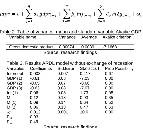
𝑔𝑑𝑝𝑟 = 𝑐 + ∑ 𝛼𝑗 𝑞

𝑗=1

𝑔𝑑𝑝𝑟𝑡−𝑗+ ∑ 𝛽𝑖 𝑝

𝑖=𝑚

𝑖𝑛𝑓𝑖−𝑚+ ∑ 𝛿𝑔 𝑦

𝑔=𝑛

𝑚2𝑔𝑔−𝑛+ 𝜔𝑡

Table 2. Table of variance, mean and standard variable Akaike GDP Variable name Variance Average Akaike criterion Gross domestic product 0.00074 0.0039 -7.1668

Source: research findings

Table 3. Results ARDL model without exchange of recession Variables Coefficients Std.Error Statistics t Prob Possibility Intercept 0.003 0.007 0.417 0.67

GDP (1) -0.61 0.08 -7.03 0.00 GDP (2) -0.65 0.07 -8.66 0.00 GDP (3) -0.63 0.08 -7.07 0.00 Inf (1) 0.06 0.03 1.73 0.08 M 0.12 0.13 0.93 0.35 M (1) 0.09 0.14 0.64 0.52 M (2) 0.06 0.13 0.47 0.63

0σ 0.012 0.001 10.6 0.00

P00 0.93

P01 0.49

The results in Table 2 contains the coefficients of the variables GDP growth regime, inflation and money supply at various intervals shown. Intercept on the diet regime that reflects positively to 0.06 and is thriving. Variable coefficients GDP (GDP) is negative and significant in all three intervals. The first variable is negative and significant coefficient of the inflation gap and variable rate of money supply without interruption and at intervals of one and two are negative and significant. So between all variables of GDP, inflation and monetary are significant effect on the dependent variable (GDP). Variance of latency (zero regime) 0σ estimated to 012/0 and the boom (diet A) 1: σ is equal to 0.000, indicating that the variance of the recession is greater than the variance boom boom swing is less.

Table 4. Results Currency ARDL model without a boom Variables Coefficients Std.Error Prob Possibility Intercept 0.06 1.41 0.00

GDP (1) -1.17 1.92 0.00 GDP (2) -1.13 1.71 0.00 GDP (3) -0.63 1.65 0.00 Inf (1) -0.14 1.46 0.00 M -0.49 1.56 0.00 M (1) -0.75 1.6 0.00 M (2) 0.49 1.66 0.00

1σ 0.0000 - 0.99

P10 0.06

P11 0.5

Estimated transition probability matrix for the boom and recession regimes as follows:

P = [p00 p01_{p10 p11}] = [0.93 . 49 . 06 . 50]

The transition probability matrix represents the probability that a recession tend to stay in the same situation, the recession has been estimated that 93 percent to P00 And the probability of recession is transferred to the boom P01 is equal to 49% And the probability that the boom tends to remain in its current state of development of P11 is equal to 50% And also tend to make the transition to the recession will boost P10 is equal to 6%. So according to the transition probability matrix concluded that the downturn in the business cycle of the country is more stable. Markov switching model can also assist in the transition probability matrix average remaining period of stagnation or stay in the boom may be achieved.

The average stay in recession = 1 1−p00=

1

(7)

273

The average stay in the boom = 1

1−p11 = 1

1−0.5= 2

The above results indicate that, Average remaining period of stagnation 28/14 years and the average stay in the boom period of 2 years.

ARDL model with Currency

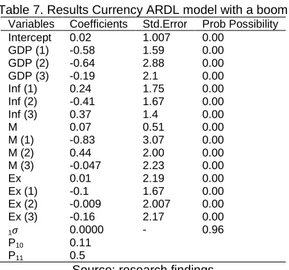
In this section the results of the Markov Suiching model ARDL enter the exchange rate in the model is given. This is results in stagnation regime (zero regime) and prosperity (one regime). Table 3 contains the results of a recession regime coefficients of the variables GDP, inflation, monetary and exchange rate at different intervals shown. Intercept the recession regime against -0.007 and is non-significant. Variable coefficients GDP (GDP) is negative and significant in all three intervals. Positive inflation differential in all three intervals, but only in the third gap is significant. Variable rate of money supply without interruption and the interruption of the first and second and third positive but only in the third gap is significant. Uninterrupted and interrupted the exchange rate variable in the first, second and third in the model Negative in all interrupts except the first break and will only be meaningful exchange without interruption.

𝑔𝑑𝑝𝑟 = 𝑐 + ∑ 𝛼𝑗 𝑞

𝑗=1

𝑔𝑑𝑝𝑟𝑡−𝑗+ ∑ 𝛽𝑖 𝑝

𝑖=𝑚

𝑖𝑛𝑓𝑖−𝑚+ ∑ 𝛿𝑔 𝑦

𝑔=𝑛

𝑚2𝑔𝑔−𝑛+ ∑ 𝛾𝑣 𝑘

𝑣=𝑙

𝑒𝑥𝑔𝑣−𝑙+ 𝜀𝑡

Table 5. Table of variance, mean and standard variable Akaike GDP Variable name Variance Average Akaike criterion Gross domestic product 0.00074 0.0039 -8.4879

Table 6. Table ARDL model results with the exchange rate in recession Variables Coefficients Std.Error Statistics t Prob Possibility Intercept -0.007 0.01 -0.6 0.49

GDP (1) -0.67 0.11 -5.8 0.00 GDP (2) -0.62 0.11 -5.3 0.00 GDP (3) -0.64 0.14 -4.42 0.00 Inf (1) 0.03 0.04 0.65 0.51 Inf (2) 0.02 0.04 0.55 0.58 Inf (3) 0.07 0.04 1.72 0.09 M 0.23 0.19 1.24 0.22 M (1) 0.13 0.17 0.78 0.43 M (2) 0.03 0.14 0.26 0.79 M (3) 0.3 0.14 2.11 0.04 Ex -0.15 0.05 -2.7 0.01 Ex (1) 0.2 0.12 1.61 0.11 Ex (2) -0.14 0.1 -1.4 0.17 Ex (3) -0.044 0.07 -0.6 0.54

0σ 0.01 0.001 9.92 0.00

P00 0.88

P01 0.49

(8)

274

Table 7. Results Currency ARDL model with a boom Variables Coefficients Std.Error Prob Possibility Intercept 0.02 1.007 0.00

GDP (1) -0.58 1.59 0.00 GDP (2) -0.64 2.88 0.00 GDP (3) -0.19 2.1 0.00 Inf (1) 0.24 1.75 0.00 Inf (2) -0.41 1.67 0.00 Inf (3) 0.37 1.4 0.00 M 0.07 0.51 0.00 M (1) -0.83 3.07 0.00 M (2) 0.44 2.00 0.00 M (3) -0.047 2.23 0.00 Ex 0.01 2.19 0.00 Ex (1) -0.1 1.67 0.00 Ex (2) -0.009 2.007 0.00 Ex (3) -0.16 2.17 0.00

1σ 0.0000 - 0.96

P10 0.11

P11 0.5

Estimated transition probability matrix for boom and bust in exchange rate regimes as follows:

P = [p00 p01_{p10 p11}] = [0.88 . 49 . 11 . 50]

The transition probability matrix represents the probability that a recession tend to stay the same recession has been estimated P00 to 88% And the probability of recession is transferred to the boom P01 is equal to 49% And the probability that the boom tends to remain in its current state of development of P11 is equal to 50% And also tend to make the transition to the recession will boost P10 to 11 percent. Thus, according to the transition probability matrix model with exchange concluded that The downturn in the business cycle of the country is more stable. The average remaining period of stagnation or stay in the boom can be obtained as follows:

The average stay in recession = 1 1−p00=

1

1−0.88= 8.33 The average stay in the boom = 1

1−p11 = 1

1−0.5= 2

The above results indicate that, Average remaining period of stagnation 33/8 years and the average stay in the boom period of 2 years.

VAR model to test linear VAR model with one or two threshold

This test is an extension of linear multivariate test of Hansen (1991) has been proposed by Lu and Zivot. The results shows that there is a linear VAR model against a threshold VAR model with a threshold rejected But there are two thresholds confirmed. Thus the study of the dynamics of the relationship between inflation and economic growth in the form of a VAR model with a threshold limit is superior to the linear VAR.

Table 8. Table test threshold VAR model Significant level _𝜒2 Statistics (0.0000) 23.7266** LR

** Significant level %5

(9)

275

Chart 1

The results of estimating a threshold VAR model

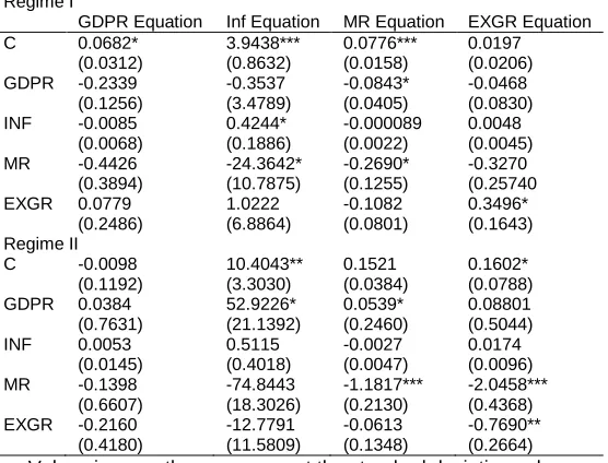
Threshold VAR model helps us to establish a causal relationship between economic growth and inflation variables in different regimes examined. For this purpose, at the threshold of a four-variable models, three univariate and bivariate relationship between variables are used. The results of the four-variable threshold VAR model is given in the table. As the table shows the results of the equation GDPR none of the coefficients are significant variables. The exchange rate has removed from the model and to investigate the relationship between money supply, inflation and GDP will be discussed.

Table 9. The results of the four-variable VAR model eve Regime I

GDPR Equation Inf Equation MR Equation EXGR Equation C 0.0682*

(0.0312) 3.9438*** (0.8632) 0.0776*** (0.0158) 0.0197 (0.0206) GDPR -0.2339

(0.1256) -0.3537 (3.4789) -0.0843* (0.0405) -0.0468 (0.0830) INF -0.0085

(0.0068) 0.4244* (0.1886) -0.000089 (0.0022) 0.0048 (0.0045) MR -0.4426

(0.3894) -24.3642* (10.7875) -0.2690* (0.1255) -0.3270 (0.25740 EXGR 0.0779

(0.2486) 1.0222 (6.8864) -0.1082 (0.0801) 0.3496* (0.1643) Regime II

C -0.0098 (0.1192) 10.4043** (3.3030) 0.1521 (0.0384) 0.1602* (0.0788) GDPR 0.0384

(0.7631) 52.9226* (21.1392) 0.0539* (0.2460) 0.08801 (0.5044) INF 0.0053

(0.0145) 0.5115 (0.4018) -0.0027 (0.0047) 0.0174 (0.0096) MR -0.1398

(0.6607) -74.8443 (18.3026) -1.1817*** (0.2130) -2.0458*** (0.4368) EXGR -0.2160

(0.4180) -12.7791 (11.5809) -0.0613 (0.1348) -0.7690** (0.2664) - Values in parentheses represent the standard deviation values.

- Signs *, ** and *** indicate significant coefficients, respectively, at 10%, 5% and 1% respectively.

The results in Table, The three variables suggests that despite the changing amount of money, inflation and GDP in equation variable GDPR significant amount of money and inflation are And GDPR only affect GDP is interrupted by two. Since the main objective of this research is to investigate the causality between GDP and inflation , That is why the monetary variable excluded from the model and the model with the variables inflation and GDP respectively.

0 5 10 15 20 25

0 .0 0 0 .1 0 0 .2 0

Test linear VAR vs 1 threshold TVAR

LRtest12 D e n si ty

Asymptotic Chi 2 Bootstrap Test value

0 10 20 30 40

0 .0 0 0 .0 6 0 .1 2

Test linear VAR vs 2 thresholds TVAR

LRtest13 D e n si ty

(10)

276

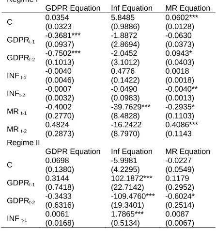
Table 10. Tuesday threshold variable VAR model estimation results Regime I

GDPR Equation Inf Equation MR Equation C 0.0354

(0.0323

5.8485 (0.9886)

0.0602*** (0.0128) GDPRt-1 -0.3681*** _(0.0937) -1.8872 _(2.8694) -0.0630 _(0.0373)

GDPRt-2 -0.7502*** (0.1013) -2.0452 (3.1012) 0.0943* (0.0403) INF t-1 -0.0040

(0.0046) 0.4776 (0.1422) 0.0018 (0.0018) INFt-2 -0.0007 (0.0032) -0.0490 (0.0983) -0.0040** (0.0013) MR t-1 -0.4002

(0.2770)

-39.7629*** (8.4828)

-0.2935* (0.1103) MR t-2

0.4824 (0.2873) -16.2422 (8.7970) 0.4086*** (0.1143 Regime II

GDPR Equation Inf Equation MR Equation C 0.0698

(0.1380) -5.9981 (4.2295) -0.0227 (0.0549) GDPRt-1 0.3144 (0.7418) 102.1872*** (22.7142) 0.1179 (0.2952) GDPRt-2 -0.3433 (0.6316) -109.4760*** (19.3401) -0.6024* (0.2514) INF t-1 0.0061 _(0.0168) 1.7865*** _(0.5134) 0.0087 _(0.0067)

For the purposes of this section, a bivariate threshold model is used to examine the relationship between variables. The results of the estimation of the VAR model is given in Table threshold.

Table 11. Results threshold bivariate VAR model

Variables GDPR Equation Inf Equation GDPR Equation Inf Equation Regime I Regime II

C 0.0646*** (0.0158) 2.3099** (0.7690) 0.0563 (0.1175) 36.6157*** (5.7178) GDPRt-1 -0.8229*** (0.0856) -4.0165 (4.1667) 0.4923 (1.8557) 518.6541*** (90.3111) GDPRt-2 -0.9545***

(0.0746) 1.2445 (3.6313) -0.8671 (0.7671) -18.5006 (37.3425) GDPRt-3 -0.7278*** (0.0890) -6.0054*** (4.3337) -0.4656 (0.9940) 179.8353*** (48.3874) inft-1 -0.0073*

(0.0031) 0.3117* (0.1505) 0.0116 (0.0127) 0.2539 (0.6179) inft-2 0.0005 _(0.0022) -0.1620 _(0.1086) -0.0101 _(0.0146) -1.0479 _(0.7119)

inft-3 -0.0002 (0.0020) 0.3024** (0.0959) -0.0139 (0.0259) -5.2053*** (1.2597)

(11)

277

Chart 2. Results of the variable threshold

The plot revolves around a threshold value calculated trend inflation (7.71) is shown. As the diagram above the level of inflation during the period 1992 - 2010 has been a lot of volatility, The highest level of inflation is for the year 1994 show few signs of inflation in 2004. Only in 200200: 4 levels of inflation will be calculated according to a threshold level. During the period 1992 - 1995 inflation is above the threshold level fluctuates but from 1996 onwards the inflation rate is below the threshold level of inflation.

.

CONCLUSION

According to the main findings of the survey results can be explained as follows. Test results of the VAR model with linear VAR model showed that there were one or two threshold linear VAR model against a threshold VAR model with a threshold rejected But there are two thresholds confirmed. Thus the study of the dynamics of the relationship between inflation in the form of a VAR model with a threshold limit is superior to the linear VAR.

The results showed that the threshold vector pattern autoregressive threshold value calculated in 7.71 inflation is estimated. The 88.7% of observations in regime (inflation below the threshold level) and 11.3% of observations in regime (inflation above the threshold level) are located. In each regime INF and GDPR two equations are estimated for GDP and inflation.The rate of inflation has meaning only in the first interval. This shows that when inflation is lower than a threshold value (regime) with an interval variable inflation can have a significant impact on economic growth. Second and third lags of inflation have a significant effect on economic growth. It should be noted that the theoretical framework of research in inflation below the threshold will have a positive impact on economic growth According to the results obtained in the economy and this is not true in the study And only second interval is a positive factor which can not have a solid base for the non-certified interface inflation and economic growth.

GDP differential equation in the regime of inflation in the first interruption positive and negative sign in the second and third intervals Which indicates that the interrupt with inflation above the threshold (7.71), economic growth is reduced. Figures based on variable threshold level of inflation during the period 1992 - 2010 has been a lot of volatility, The highest level of inflation for 1994 and 2004 is at least the level of inflation. Only in 2004: 4 levels of inflation will be calculated according to a threshold level. During the period 1992 - 1995 inflation is above the threshold level fluctuates but from 1996 onwards the inflation rate is below the threshold level of inflation.

In summarizing the results of the VAR model can be stated threshold The threshold level of inflation for the economy and inflation 7.71 percent is estimated that currently there's a huge difference.

Time

0 10 20 30 40 50 60 70

0

5

10

15

20

Threshold variable used

th 1

0 10 20 30 40 50 60 70

0

5

10

15

20

Ordered threshold variable

trim= 0.1 th 1

2 3 4 5 6 7 8

440

480

520

Threshold Value

SSR

Results of the grid search

(12)

278

REFERENCES

Amisano G & Fagan G. 2013. Money growth and inflation: A regime switching approach, journal of international money and finance ,Volume 33, pp: 118–145.

Coibion O, Gorodnichenko Y & Wieland J. 2011. The Optimal Inflation Rate in New Keynesian Models:Should Central Banks Raise Their Inflation Targets in Light of the Zero Lower Bound?, working paper.

Dashti SA. 2007. Relationship between inflation and economic growth in Iran. Bureau of Economic Research, Department of Macroeconomics, 20-6.

Fountas S, Karanasos M & Kim J. 2002. Inflation and output growth uncertainty and their relationship with inflation and output growth. Economics Letters, 75 (3), 293-301.

Hasanov F. 2011. Relationship between inflation and economic growth in Azerbaijani economy: is there any threshold effect?, Institute for Scientific Research on Economic Reforms, Ministry of Economic Development of the Republic of Azerbaijan, MPRA Paper No. 33494.

Mandler M. 2010. Macroeconomic dynamics and inflation regimes in the U.S. Results from threshold vector auto regressions. Joint Discussion Paper Series in Economics No. 12.

Mubarik YA. 2005. Inflation and growth: An estimate of the threshold level of inflation in Pakistan, SBPRes, Bull. 1, PP: 35-44. Peraei ST and Dadvar B. 2011. The effect of inflation on economic growth in the country with an emphasis on the uncertainty.

Research Paper, No. 1, pages 80-67.

Peraei ST and Dadvar B. 2011. The effect of inflation on economic growth in the country with an emphasis on the uncertainty. Research Paper, No. 1, pages 80-67.

Kremer S, Bick A & Nautz D. 2011. Inflation and Growth: New Evidence from a Dynamic Panel Threshold Analysis. Working Paper, Free University Berlin, Department of Economics, Boltzmannstr.