Sub-pixel Edge Detection of LED Probes Based On Partial Area Effect

─────────────────────────

Sub-pixel Edge Detection of LED Probes Based On

Partial Area Effect

Chung-Yen Su

, Li-An Yu

, Nai-Kuei Chen

, Jheng-Jyun Wang

, Ying-Hao Liu

, Shuen-De Wu

1

_{Department of Electrical Engineering,}

_{Department of Mechatronic Engineering}

National Taiwan Normal University, Taiwan

[email protected], [email protected], [email protected], [email protected],

[email protected], [email protected]

Abstract—In recent years, the demands for LED are

increasing. For testing the quality of LEDs, a lot of LED probes are necessary, so the high precision and efficient methods are paid more attention by industrial applications. This paper is focused on the measurement of the angle and the radius of a LED probe by computer vision. In previous paper, we proposed an effective method based on Canny edge detection and curve fitting method with iteration. In this paper we add a new sub-pixel edge detection method: partial area effect. We improve the preciseness of angle from error 2.3% to 1.43% and enhance the accuracy of radius more than 30%.1

Keywords—Edge detection, Sub-pixel edge detection, Probe, LED

I. INTRODUCTION

Edges are always in high frequency and located in high contrast region. Edge detection is the crucial step for many computer vision applications. Utilizing the characteristics of edges can help us to extract the objects from images, so determining the edge location fast and accurately is the main point for a measuring system.

The precision and accuracy is the main target of measuring LED probes. In order to test a LED probe’s angle and radius, as shown in Fig. 1, the input images from camera have to be processed, including filtering, edge detection, sub-pixel edge detection, and so on.

Detecting the edge of a LED probe generally has the following five main steps.

Step 1: Use a low-pass filter to reduce the noise.

Step 2: Detect coarse edge points by a pixel level edge detection.

Step 3: Classify the coarse edge points to get three groups. Two groups of them are used to estimate the angle and one is used to estimate the radius, respectively. Step 4: Use a sub-pixel edge detection to improve the

coarse edge points.

Step 5: Use the curve fitting algorithm to determine the angle and the radius.

1 _{This work is partly supported by National Science Council under Contract}

No. NSC 102-2218-E-003-001-MY2

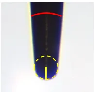
Fig. 1. The solid lines with red and yellow are angle and radius of a LED probe, respectively.

The commonly used filters to reduce noise are mean filters and Gaussian filters [1, 2]. Coarse edge detection can be performed by using the general operators including Sobel, Scharr, Laplacian of Gaussian (LOG), and Canny. These operators are efficient on edge detection, but the positions of detected edge points are all in pixel level.

To increase the precision of edge detection, several sub-pixel techniques had been proposed, including curve-fitting, moment-based [3-6], reconstructive [7] and partial area effect methods [8]. These methods have their characteristics. Curve-fitting methods are computationally simple but are easily affected by noise. Moment-based methods use integral pixels to reduce the effect of noise but require more computations. Reconstructive methods use horizontal gradients or vertical gradients to build a curve and find the peak of the curve as the sub-pixel edge. Partial area effect methods require different sizes of blocks to serve as horizontal and vertical models.

In literature, Tabatabaic and Mitchell were first two people to use sub-pixel technique to increase precision of edge detection. In [3], a Zernike orthogonal moment-based (ZOM) method is proposed for sub-pixel edge detection. The property of ZOM is rotation invariant and it is useful for pattern recognition and matching. In [4], Bin et al. proposed a method of detecting sub-pixel edges based on Fourier-Mellin Moment (OFMM). This method has a great ability to describe tiny things. In order to reduce the computational complexity, some researchers used Sobel operator to determine coarse edges before using moment-based sub-pixel methods [5, 6]. Recently, Trujillo-Pino et al. [8] proposed a new sub-pixel detection method based on partial area effect and showed that it is effective for camera captured images with apparent boundary. Motivated by the partial area effect method, we add it to our previous method [9] and then compare its results with other

INISCom 2015, March 02-04, Tokyo, Japan Copyright © 2015 ICST

sub-pixel methods. Finally, we conclude the better method for measuring the LED probes.

This paper is organized as follows. Section 2 consists of the basic information about sub-pixel edge detection. Section 3 details the proposed method. Section 4 shows the experimental results with three different methods. We make the concluding remarks in the last section.

II.SUB-PIXEL EDGE DETECTION

Although edge-detection methods can get the coarse edges of an object, the level of the edge information is in pixel. In order to enhance the precision of edge points, we use sub-pixel techniques, including iterative curve-fitting and partial area effect methods. We briefly introduce these sub-pixel edge detections as follows.

A. Iterative curve-fitting

For a curve-fitting method, we build a model by using edge points (see Fig. 2). Let the sum of squared errors between the edge points and the model be the smallest. Then the model is the best fit to these edge points. It is easy to compute the parameters of the model.

Fig. 2. Blue line shows the best fit of the edge points.

In order to reduce the effects of badly defined edge points on straight line, we calculate the standard deviation with the equation of line L1 which is calculated by curve-fitting method at first. Then we eliminate the points which are far from L1 (larger than two times of standard deviation). After that, the model of the best fit is recalculated. This process continues until the maximum number of iteration is reached or no more points are eliminated. We called the process as iterative curve-fitting method. With the iterative curve-curve-fitting method, we can get a more accurate straight line than the first one we got. B. Partial area effect

We briefly introduce the method based on partial area effect herein. More details can refer to [8]. At first, we create the 3 ×

9 mask for the selected edge point and calculate dx and dy by Sobel operator to get the value of m, as shown in the following expressions.

m = 1 if dx×dy > 0 (1)

m = -1 if dx×dy < 0 (2)

Next, two constraints (see (3) and (4)) are used to check if one point’s gradient is the local maximum or not. If the answer is yes, the direction of mask type is determined by comparing the values of |dx|and |dy|.

Constraint 1:

|𝑑𝑥(𝑥 − 1, 𝑦)| ≤ |𝑑𝑥| AND |𝑑𝑥| ≥ |𝑑𝑥(𝑥 + 1, 𝑦)| (3) Constraint 2:

|𝑑𝑦(𝑥, 𝑦 − 1)| ≤ |𝑑𝑦| AND |𝑑𝑦| ≥ |𝑑𝑦(𝑥, 𝑦 + 1)| (4)

Mask type Linear equation Condition

Vertical: 𝑦 = 𝑎 + 𝑏𝑥 + 𝑐𝑥2 _{|dy| > |dx|} Horizontal: 𝑥 = 𝑎 + 𝑏𝑦 + 𝑐𝑦2 _{|dx| > |dy|}

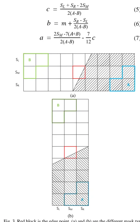
If the mask type is vertical (|dy|>|dx|), the y of x equation is used. Otherwise, the x of y equation is used instead. Each equation is assumed as a linear equation, as shown as above. The parameters (𝑎, 𝑏 and 𝑐) of each linear equation can be calculated from A, B, SL, SMand SR (see (5)-(7)). A and B are the average intensities of blue and green ranges in Fig. 3, respectively. SL, SM, and SR are the sum of intensities of the row in Fig. 3(a) or column in Fig. 3(b).

c

=

2(A-B) (5)

b

=

a

=

2(A-B) - 7

12

c

SL

SM

SR A

B

(a)

SL SM SR

B

A

(b)

Fig. 3. Red block is the edge point. (a) and (b) are the different mask type of partial area effect method.

y

x

Finally, we can get the sub-pixel position of the edge point according to different mask type, as shown as below.

Mask type Sub-pixel position Vertical: (x, y + a) Horizontal: (x + a, y)

III. PROPOSED METHOD

At first, we briefly introduce our previous method [9]. Then, we depict the differences between the previous method and the proposed method.

In [9], we reduced the noise by using a mean filter to the gray-level images captured from the camera. Next, we used Canny edge detection to get coarse edges and Sobel operator to compute gradient directions. The directions are used to classify the edge points into three groups, namely left line group, right line group, and circle group. Finally, we used the aforementioned iterative curve-fitting method to calculate the angle and the radius of a LED probe.

Start

Gaussion Filter

Canny Edge Detection

Object Extraction

Use Sobel

Operator to Getq. q = tan-1(dy/dx)

For line: |q|<7 For circle: |q|>30

Partial Area Effect Method

Iterative

Curve-fitting to Get Angle and

Radius

End

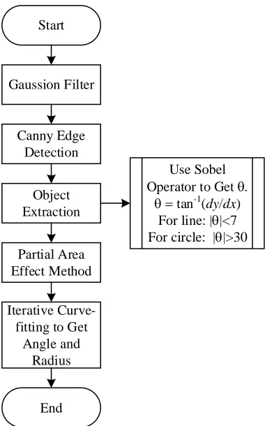
Fig. 4. Flow chart of the proposed method.

Figure 4 shows the flow chart of the proposed method. We replace the mean filter by a 55 Gaussian filter. We still use Canny edge detection to find the coarse edge points but set its high and low thresholds automatically to increase the efficiency during processing. We calculate the mean intensity of a gray image and multiply the mean intensity by 0.3 to serve

as the high threshold and by 0.1 to serve as the low threshold, respectively.

The coarse edge points will be classified into three groups. First, we use the middle position of the probe to separate the points into right points and left points. Next, we get the gradient direction q of each point from Sobel operator by using

θ = tan−1 𝑑𝑦

𝑑𝑥 (8) where

𝑑𝑥 = 𝑓(𝑖, 𝑗) ∗ [

−1 0 1 −2 0 2 −1 0 1

]

and

𝑑𝑦 = 𝑓(𝑖, 𝑗) ∗ [

−1 −2 −1 0 0 0 1 2 1

].

Herein, f(i, j) denotes the image pixel value and the notation “*” denotes the convolution.

Compared with the previous method [9], the proposed method modifies the conditions in the object extraction. The new conditions are as follows. If the absolute value of a point’s direction is smaller than 7 degree, |𝜃| < 7∘, the point is classified into the line groups. On the other hand, if the absolute value of a point’s direction is above 30 degree, |𝜃| > 30∘, the point is classified into the circle group (the front of a probe). A point that does not fit these two conditions is discarded. Note that these conditions are made by the experiment. We found that a vertically placed probe has an angle, which is always smaller than 14∘, as shown in Fig. 5. By using the proposed conditions, we can get the three groups of edge points for a real probe, as illustrated in Fig. 6.

14° 7°

Right

line

Left

line

Circle

30°

Fig. 5. The gradient directions of lines and the front of the probe.

Fig. 6. Left line, right line and circle groups are illustrated in red, orange and blue colors, respectively.

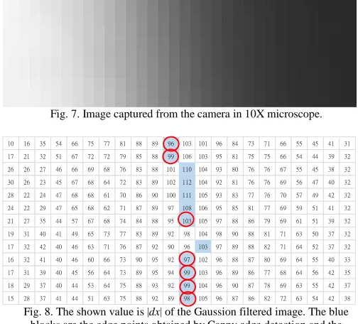
and occupies a wide range, as shown in Fig. 7. With the two constriants, many non-local maximum edge points will be eliminated. For example, there are twelve edge points found from the Canny edge detection as shown in Fig. 8 and seven of them are elimated from the constraint in (3).

Fig. 7. Image captured from the camera in 10X microscope.

Fig. 8. The shown value is |dx| of the Gaussion filtered image. The blue blocks are the edge points obtained by Canny edge detection and the

blocks with a red circle will be eliminated with the two constraints.

Finally, we use the iterative curve-fitting method to get two linear equations (see (9) and (10)). One is calculated from the points in the left line group, and the other is calculated from the points in the right line group.

Left line: 𝑦 = 𝑚1𝑥 + 𝑒 (9)

Right line: 𝑦 = 𝑚2𝑥 + 𝑓 (10)

where m1 and m2 are the slopes of the lines, and e and f denote the corresponding intercepts.

After getting these parameters of lines, we can get the angle of the probe by using the cosine theorem.

𝜃 = cos−1_(| 𝑚1×𝑚2+1

√𝑚12+1×√𝑚22+1|) (11)

As for the radius, we build a circle model from the points in the circle group. The circle model is shown in (12). With it, we can get the radius of the probe from (13).

Circle model: 𝑥2_{+ 𝑦}2_{+ 𝑑𝑥 + 𝑒𝑦 + 𝑓 = 0 (12)}

Radius: 𝑅 =1

2√𝑑

2_{+ 𝑒}2_{− 4𝑓 (13)}

IV. EXPERIMENTAL RESULTS

In the experiment, we have 23 test images that are captured by a CMOS sensor camera. The size of the images is 19201080. Some of the images are shown in Fig. 9. Since these images are captured in BGR format, we need to transform them to get their corresponding grey-level images first. Then we use the proposed method to calculate the angle and the radius of each LED probe. We set the maximum numberof iteration in the iterative curve-fitting method to five. Table I tabulates the experimental results. In the table, we also list the results of [8] and [9] for comparison. The referred values are measured from a SEM (Scanning Electron Microscope) system. For the step of sub-pixel edge detection, the proposed method is different from [8] in the two constraints. We do not use these two conditions to avoid removing too much points, leading to a worse result. For clarity, we mark the best values of angle error and radius error for each sample image in red digits.

As we can see in the table, the proposed method generates most of the best results. The average angle errors are 2.3% for [9], 1.54% for [8], and 1.43% for the proposed method, respectively. Thus, the proposed method has the smallest average angle error. As for the average radius errors, they are 37.22% for [9], 1.61% for [8], and 1.43% for the proposed method, respectively. Likely, the proposed method has the smallest average radius error. Note that the method in [9] has a quite large radius error because it uses a different scheme to determine the thresholds of Canny edge detection and it does not use any sub-pixel edge detection to refine the locations of edge points.

(a) (b) (c) (d)

(e) (f) (g) (h)

Fig. 9. (a), (b), (c), (d), (e), (f), (g) and (h) are samples from 1 to 8, respectively

V.CONCLUSION

In this study, we proposed a method to determine the edge locations with sub-pixel accuracy for the application of LED probes. In the proposed method, we use Canny edge detection to find coarse edge points after using a Gaussian filter to reduce the noise. Next, we classify the points into three groups and discard remaining points. We refine the edge location of each point by using the partial area effect method without two constraints. Finally, we calculate the angle and the radius of a probe by using the iterative curve-fitting. Experimental results show the effectiveness of the proposed method.

10 16 35 54 66 75 77 81 88 89 96 103 101 96 84 73 71 66 55 45 41 31

17 21 32 51 67 72 72 79 85 88 99 106 103 95 81 75 75 66 54 44 39 32

26 26 27 46 66 69 68 76 83 88 101 110 104 93 80 76 76 67 55 45 38 32

30 26 23 45 67 68 64 72 83 89 102 112 104 92 81 76 76 69 56 47 40 32

28 22 24 47 68 68 61 70 86 90 100 111 105 93 83 77 76 70 57 49 42 32

24 22 29 47 65 68 62 71 87 89 97 108 106 95 85 81 77 69 59 51 41 32

21 27 35 44 57 67 68 74 84 88 95 103 105 97 88 86 79 69 61 51 39 32

19 31 40 41 49 65 73 77 83 89 92 98 104 98 90 88 81 71 63 50 37 32

17 32 42 40 46 63 71 76 87 92 90 96 103 97 89 88 82 71 64 52 37 32

16 32 41 40 46 60 66 73 90 95 92 97 102 96 88 87 80 69 64 55 40 33

17 31 39 40 45 56 64 73 89 95 94 99 103 96 89 86 77 68 64 56 42 35

18 29 37 40 44 53 64 75 88 93 92 99 104 96 90 87 78 69 63 55 42 37

Table 1 Experimental results of different sub-pixel edge detection methods

Referred values [9] [8] Proposed method

Items

Image

Angle (degree)

R (um)

Angle Error (%)

Radius Error (%)

Angle Error (%)

Radius Error (%)

Angle Error (%)

Radius Error (%)

sample1 10.1 16.75 1.98 14.09 1.97 0.55 1.91 0.01

sample2 10.3 20.75 1.65 100 1.1 2.1 0.96 2.17

sample3 10.2 21.25 2.06 0.85 2.43 0.9 1.91 3.06

sample4 10.3 15.25 1.94 8.72 1.76 0.47 1.36 0.79

sample5 10.7 23.25 0.75 12.47 0.44 4.49 0.11 1.91

sample6 9.6 25.25 1.98 3.25 0.57 0.16 0.6 0.27

sample7 10.5 22.25 0.76 41.44 1.13 1.78 1.09 1.91

sample8 10.4 22.75 0.87 20.22 0.52 2.43 0.42 2

sample9 10.1 23.25 2.87 11.78 1.83 2.56 1.77 3.68

sample10 10.1 22.25 2.57 91.51 1.79 0.54 1.64 0.01

sample11 9.4 22.75 3.83 1.23 3.61 0.89 3.39 0.06

sample12 10.2 24.75 1.18 76.32 0.36 0.81 0.16 0.26

sample13 10.1 23.75 1.98 24.59 1.86 1.54 1.52 0.02

sample14 10 21.25 2.3 13.13 1.8 0.16 2.1 1.1

sample15 10.1 23.75 1.78 100 1.45 2.35 1.61 2.21

sample16 10.7 23.75 3.18 56.63 2.27 6.83 2.28 7.04

sample17 10.3 22.75 0.29 19.6 0.17 0.41 0.3 0.75

sample18 10.2 23.25 3.14 87.53 3.17 0.66 3.01 0.67

sample19 9.7 23.75 10.72 100 0.34 1.15 0.21 1.15

sample20 10.2 23.25 2.75 22.75 2.4 2.64 2.15 1.99

sample21 9.7 22.25 0.62 10.65 0.61 1.62 0.81 0.79

sample22 10.3 22.25 2.23 7.55 1.9 0.73 1.69 0.61

sample23 9.8 23.75 1.53 31.83 2 1.33 1.91 0.47

REFERENCES

[1] R. C. Gonzalez and R. E. Woods, “Digital Image Processing,” 3rd _Edition,

Prentice-Hall, Inc., 2008.

[2] R. C. Gonzalez, R. E. Woods, and S. L. Eddins, “Digital Image

Processing-using MATLAB,” Edition, Prentice-Hall, Inc., 2004.

[3] S. Ghosal, R. Mehrota, “Orthogonal moment operators for subpixel edge

detection,” Pattern Recognition, 26 (2), pp.295-306, 1993.

[4] T. J. Bin, A. Lei, J. W. Cui, W. J. Kang, D.D. Liu, “Subpixel edge

location based on orthogonal Fourier-Mellin moments,” Image and

Vision Computing, 26 (4), pp. 563-569, 2008.

[5] Y. D. Qu, C. S. Cui, S. B. Chen, J. Q. Li, “A fast subpixel edge detection

method using Sobel-Zernike moments operator,” Image and Vision

Computing, 23 (1), pp. 11–17, 2005.

[6] Z. F. Hu, H. S. Dang, X. R. Li, “A novel fast subpixel edge detection

method based on Sobel-OFMM, ” in Proc. of IEEE International

Conference on Automation and Logistics, pp. 828-832, 2008.

[7] A. Fabijańska, “A survey of subpixel edge detection methods for images

of heat-emitting metal specimens,” International Journal of Applied Mathematics and Computer Science, vol. 22, no. 3, pp. 695-710, 2012.

[8] A. Trujillo-Pino, K. Krissian, M. Alemán-Flores, D. Santana-Cedrés,

“Accurate subpixel edge location based on partial area effect”, Image and Vision Computing, 31, pp. 72–90, 2013.

[9] N. Q. Chen, J. J. Wang, L. A. Yu, and C. Y. Su, “Sub-pixel Edge Detection of LED Probes Based on Canny Edge Detection and Iterative

Curve Fitting”, in Proc. of IEEE International Symposium on Computer,