Derived Patterns in Binocular Rivalry Networks

DOI10.1186/2190-8567-3-6

R E S E A R C H Open Access

Derived Patterns in Binocular Rivalry Networks

Casey O. Diekman·Martin Golubitsky· Yunjiao Wang

Received: 15 January 2013 / Accepted: 22 April 2013 / Published online: 8 May 2013

© 2013 C.O. Diekman et al.; licensee Springer. This is an Open Access article distributed under the terms of the Creative Commons Attribution License (http://creativecommons.org/licenses/by/2.0), which permits unrestricted use, distribution, and reproduction in any medium, provided the original work is properly cited.

Abstract Binocular rivalry is the alternation in visual perception that can occur when the two eyes are presented with different images. Wilson proposed a class of neuronal network models that generalize rivalry to multiple competing patterns. The networks are assumed to have learned several patterns, and rivalry is identified with time peri-odic states that have periods of dominance of different patterns. Here, we show that these networks can also support patterns that were not learned, which we callderived. This is important because there is evidence for perception of derived patterns in the binocular rivalry experiments of Kovács, Papathomas, Yang, and Fehér. We construct modified Wilson networks for these experiments and use symmetry breaking to make predictions regarding states that a subject might perceive. Specifically, we modify the networks to include lateral coupling, which is inspired by the known structure of the primary visual cortex. The modified network models make expected the surprising outcomes observed in these experiments.

Keywords Binocular rivalry·Interocular grouping·Coupled systems·Symmetry· Hopf bifurcation

1 Introduction

Wilson [1] argues that generalizations of binocular rivalry can provide insight into conscious brain processes and proposes a neural network model for higher level de-cision making. Here, we demonstrate that the Wilson network model is also useful for

C.O. Diekman·M. Golubitsky (

Mathematical Biosciences Institute, The Ohio State University, Columbus, OH 43210, USA e-mail:[email protected]

Y. Wang

Fig. 1 aNecker cube illusion [7] andbrivalry [6]

understanding the phenomenon of binocular rivalry itself by analyzing several rivalry experiments discussed in Kovács, Papathomas, Yang, and Fehér [2]. Mathematical analysis of these network structures (based on the theory of coupled cell systems and symmetry in Golubitsky and Stewart [3–5]) leads to predictions that are directly testable via standard psychophysics experiments.

We begin by making a distinction between two types of perceptual alternations (Blake and Logothetis [6]):illusionsdue to insufficient information andrivalrydue to inconsistent information. One of the standard examples of illusion is given by the Necker Cubeshown in Fig.1(a). There are two percepts that are commonlyperceived when viewing the Necker cube picture: one with the yellow face at the back and one with it on top. There is not enough information in the picture to fix the percept and this ambiguity leads to the two percepts alternating randomly.

In rivalry, the two eyes of the subject are presented with two different images such as the ones in Fig.1(b) [6]. Typically, the subject reports perceiving the two images alternating in periods of dominance. There are two main types of mathematical mod-els for rivalry (Laing et al. [8]). In the first type, rivalry is treated as a time periodic state (perhaps with added noise), and in the second the oscillation is obtained by noise driven jumping between stable equilibria in a bistable system (Moreno-Bote et al. [9]).

The simplest deterministic version of the first type, studied by many authors in-cluding [1,10–18], assumes that there are two unitsaandbcorresponding to the two percepts with a system of differential equations of the form

˙

Xa=F (Xa, Xb)

˙

Xb=F (Xb, Xa)

(1)

where the vectorXaconsists of the state variables of unitaand the vectorXbconsists

of the state variables of unitb. The equations in (1) are those associated with the two-node network in Fig.2. It is further assumed that one of the variablesxE_∗ is anactivity variable and thatx_aE> x_bE implies that perceptais dominant. Similarly, perceptbis dominant ifx_bE> x_aE. In these models equilibria whereXa=Xbarewinner-take-all

states that correspond to one percept being dominant.

States whereXa=Xb are calledfusionstates. Fusion states are typically

Fig. 2 Two-node architecture modeling two units

because of the symmetry in model equations such as (1), the subspaceXa=Xb is

flow-invariant, and fusion equilibria are structurally stable.

Periodic solutions representing rivalry are most easily found in model equations (1) by using symmetry-breaking Hopf bifurcation from a fusion state. Note that the symmetry in (1) is given by permuting the two units. In such systems, there are two types of Hopf bifurcation: symmetry-preserving and symmetry-breaking. The two types are distinguished by which subspace

V+=(Xa, Xb):Xb=Xa)

or V−=(Xa, Xb):Xb= −Xa)

contains the critical eigenvectors at Hopf bifurcation. Symmetry implies that generi-cally the critical eigenvectors are either in one subspace or the other [5]. Symmetry-preserving Hopf bifurcations (with critical eigenvectors inV+) lead to periodic so-lutions satisfyingXb(t )=Xa(t ), that is, to oscillation of fusion states. These states

are perhaps uninteresting from the point of view of rivalry. Symmetry-breaking Hopf bifurcations (with critical eigenvectors inV−) lead to periodic solutions satisfying

Xb(t )=Xa(t+T₂), whereT is the period. Such solutions lead to periodic

alterna-tion between perceptsaandb; that is, to rivalrous solutions.

Kovács et al. [2] published an influential paper demonstrating that subjects can perceive alternations between coherent images even when the components of those images are scrambled and distributed between the two eyes (Lee and Blake [21]). The unscrambling of component pieces to obtain a coherent percept, termedinterocular grouping, had been documented previously (Diaz-Coneja [22] and Alais et al. [23]), and has since been reproduced using a variety of rivalry stimuli (Papathomas et al. [24]). Of the four rivalry experiments described in [2], only the first can be under-stood by the simple two-node network in Fig.2. We will show that the other three experiments can be modeled using a variant of Wilson networks for generalized ri-valry. In their first experiment, subjects are presented themonkeyandtextimages in Fig.3(a)) and they report rivalry between the two images. In their second experiment, subjects are presented the scrambled images combining parts of the monkey’s face and parts of the written text (see Fig.3(b)). The subjects report that, in addition to the expected rivalry between the original scrambled images, for part of the time they perceive alternations between unscrambled images ofmonkeyonly andtextonly such as those in Fig.3(a). We show that the surprising outcome of this experiment is not surprising when formulated as a simple Wilson network.

Fig. 3 From Kovács et al. [2] ©(1996) National Academy of Sciences, USA.aLearned images in mon-key-textrivalry experiment.bLearned images in scrambledmonkey-textexperiment

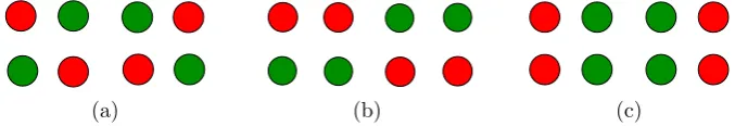
Fig. 4 From Kovács et al. [2] ©(1996) National Academy of Sciences, USA.aLearned images in con-ventionalcolored dotexperiment.bLearned images in scrambledcolored dotexperiment

Besides reporting rivalry between the two single-color figures, the subjects unexpect-edly report images with dots of scrambled colors, such as those in Fig.4(b). The corresponding result for the conventionalmonkey-textexperiment seems highly un-likely.

In the scrambledcolored dotexperiment, [2] presented the subjects with the im-ages in Fig.4(b). Given the results of the scrambledmonkey-textexperiment, it is not surprising that subjects reported rivalry between these two scrambled color images and also rivalry between single color images such as shown in Fig.4(a). However, the analogy of the scrambled colored dotexperiment with the scrambled monkey-textexperiment is not quite so straightforward, since, as we will see in Sect.2, the proposed Wilson networks for the two experiments have different symmetries.

Tong, Meng, and Blake [25] give a simplified description of thecolored dot ex-periments of [2] by using a square array of four dots rather than a rectangular array of 24 dots. Our analysis is based on the simplified 2×2 versions of these experiments, but extends to the 6×4 case.

(1) The simplest Wilson model for the conventionalmonkey-textexperiment is the standard two-node rivalry model in Fig.2and leads only to rivalry between the wholemonkeyand the wholetextimages.

(2) The simplest Wilson model for the scrambledmonkey-textexperiment leads nat-urally to rivalry solutions between the scrambled images and also between the reconstructed images.

(3) The modified Wilson model for the scrambledcolored dotexperiment also leads naturally to rivalry solutions between both the scrambled and the reconstructed images.

(4) The Wilson model for the conventionalcolored dotexperiment leads naturally to rivalry between scrambled images as well as to between the conventional images. This is in contrast to the conventionalmonkey-textexperiment.

We will see that our analysis also leads to possible additional rivalry states in the colored dotexperiments and these states may be thought of as predictions made by our approach.

The remainder of the paper is organized as follows. We describe Wilson networks in Sect.2. Our discussion differs from [1] in two important ways. First, we observe that patterns exist in rivalrous solutions for the Wilson networks that are not learned patterns. We call these additional patternsderived; the derived patterns are the ones that correspond to the unexpected results in the Kovács et al. experiments. Second, we introduce an additional type of coupling,lateral coupling, based on models of hypercolumns in the primary visual cortex literature (Bressloff et al. [26]).

Deciding on the exact form of a Wilson network model for a given experiment is not at this stage algorithmic. Moreover, there are many choices for the exact form of the network equations once the network is fixed. If we take the strict form of the Wilson models (where all nodes, all excitatory couplings, and all inhibitory couplings are identical) and we assume that the associated differential equations are highly idealized rate models (as Wilson does), then the derived patterns in themonkey-text experiment are always unstable. However, stability is a model-dependent property of solutions and simple changes to the network or to the model equations can lead to stable derived patterns.

There are many ways to modify Wilson networks to address the stability issue and we have chosen one here, namely, we have added lateral coupling to the network. Lateral coupling will also enable us to distinguish the Wilson network models for the twocolored dotexperiments by a change in network symmetry. The most important message in this paper is the observation that Wilson networks have derived patterns that can be classified using methods from the theory of symmetry-breaking Hopf bifurcations and that these derived patterns appear to correspond to the surprising perceived states found in psychophysics experiments. More discussion is needed to arrive at an algorithmic description of which (modified) Wilson network to use when modeling a given experiment.

Fig. 5 Architecture for a Wilson network.aInhibitory connections between nodes in an attribute column.

bExcitatory connections in a learned pattern.cExcitatory lateral connections

Stewart [27]) and ofD4symmetry (as in Golubitsky et al. [5]). Note thatS4 is the group of permutations on four letters andD4is the symmetry group of a square.

Section4summarizes the calculations needed to compute stability for rivalrous solutions between both learned and derived patterns in the scrambled monkey-text networks. In this section, we use standard rate models to compute stability and to illustrate the effect of having lateral coupling.

We end this Introduction by emphasizing that our approach is mainly amodel independentone advocated in Golubitsky and Stewart [4]. We use network structure and symmetry to create a menu of possible rivalrous solutions, rather than explicitly finding these solutions in a given differential equations model, such as is typically done in the literature [1,10,11,28]. This menu is model independent. Stability, on the other hand, ismodel dependent. Our discussion of stability in Sect.4does rely on the choice of specific model equations; here we use the rate models introduced by others.

2 Networks

Wilson networks [1] are assumed to have learned several patterns, and rivalry is iden-tified with time-periodic states that have periods of dominance of different patterns. Here, we show that these networks can also support derived patterns in addition to learned patterns.

A pattern is defined by the choice of levels of a set of attributes. Specifically, Wil-son networks consist of a rectangular set of nodes, arranged in columns, and two types of coupling. The columns represent attributes of an object and the rows rep-resent possible levels of each attribute. There are reciprocal inhibitory connections between all nodes in each column. See Fig.5(a). In the Wilson network a pattern is a choice of a single level in each column. If the network haslearneda particular pattern, then there are reciprocal excitatory connections between all nodes in the pat-tern. See Fig.5(b). A Wilson network can learn many patterns. When it does, there are reciprocal excitatory connections between nodes in each pattern. In our discus-sion of rivalry, we assume that the images shown to each eye are the two learned patterns.

in-Fig. 6 aDistinct areas in scrambledmonkey-textexperiment.bSchematic two-attribute two-pattern Wil-son network for scrambledmonkey-textexperiment with reciprocal inhibition in attribute columns and reciprocal excitation in learned patterns.cWilson network with reciprocal lateral excitation

spired by the hypercolumn structure of the primary visual cortex (V1). Neurons in V1 are known to be sensitive to orientations of line segments located in small regions of the visual field. Moreover, V1 consists of hypercolumns, which are small regions of V1 that correspond to specific regions of the visual field. Optical imaging of macaque V1 suggests that in each hypercolumn there are neurons that are sensitive to each ori-entation, and that neurons within a hypercolumn are all-to-all coupled (Blasdel [29]). This coupling is usually assumed to be inhibitory. Thus, when considering V1, the columns in the Wilson networks correspond to hypercolumns where the attributes are the direction of a line field at a specified area in the visual field. However, V1 imag-ing also indicates a second kind of couplimag-ing, calledlateral coupling that connects neurons in neighboring hypercolumns [26,29]. Moreover, the neurons that are most strongly laterally coupled are those that have the same orientation sensitivity [26,30], albeit at different points in the visual field. Finally, lateral coupling is usually taken to be excitatory.

With the structure of V1 as inspiration, we define an excitatory lateral coupling in the Wilson networks by connecting those nodes in different columns that correspond to thesame level. See Fig.5(c).

The scrambled monkey-text experiment can be modeled by a level, two-attribute Wilson network with two learned patterns. To specify the network, we con-ceptualize the Kovács images in Fig.3(b) as rectangles divided into two regions: one indicated by white and the other by blue in Fig.6(a). The first attribute in the network corresponds to the portion of a rectangular image in the white region and the second attribute corresponds to the portion of that rectangular image in the blue region. In the Kovács experiment, the possible levels of each attribute are the portion of themonkey image in the associated region and the portion of thetextimage in that region.

This network has four nodes, whereXij represents leveliof attributej as shown

Fig. 7 Simulations of network in Fig. 6(c) showing stable rivalry for equations in (11), where G(z)= 0.8

1+e−7.2(z−0.9),I=2,w=0.25,β=1.5,g=1,ε=0.6667. Ina,δ=0 and inbδ=0.5, where

δis the strength of the lateral coupling

X22. There are also reciprocal excitatory connections betweenX11andX22and be-tweenX21 andX12 representing the two learned patterns. In this network, the state {xE₁₁> x₂₁E andx₂₂E > x₁₂E} corresponds to the scrambled image in Fig.3(b)(left), whereas the state {x₂₁E > x₁₁E and x₁₂E > x₂₂E} corresponds to the scrambled im-age in Fig.3(b)(right). Importantly, the network also supports two derived pattern states: {x₁₁E > x₂₁E andx₁₂E > x₂₂E}, which corresponds to themonkeyonly image in Fig.3(a)(left), and {x₂₁E > x₁₁E andx₂₂E > x₁₂E}, which corresponds to thetext only image in Fig.3(a)(right).

Note that lateral coupling changes the network in Fig.6(b) to the one in Fig.6(c). Simulations of the equations associated with the network in Fig.6(c) show stable rivalrous solutions between both learned and derived patterns (see Fig. 7). These simulations use the standard rate equations (11) introduced in Sect.4.

The symmetries of the networks in Fig.6(b) and6(c) are the same. Hence, for this experiment, the addition of lateral coupling does not change the expected types of periodic solutions that can be obtained through symmetry-breaking Hopf bifurcation. However, lateral coupling does change the symmetry of the Wilson network (and hence the expected types of solutions) corresponding to the scrambledcolored dot experiment as shown in Fig.9.

Tong et al. [25] suggest a simplified version of thecolored dotexperiments in [2], where each eye is presented with a square symmetric pattern of four dots. So, in the Tong version of the conventionalcolored dotexperiment, one learned pattern has four red dots and the other has four green dots, as shown in Fig.8(a). To our knowledge, this proposed rivalry experiment has not been performed.

Fig. 8 aImages in simplification of the conventionalcolored dotexperiment in [2,25].bNetwork with two learned patterns corresponding to the simplified experiment; symmetry group isΓ =S4×Z2(ρ). UL=upper left,LL=lower left,LR=lower right,UR=upper right

Fig. 9 aImages in simplification of the scrambledcolored dotexperiment in [2,25].bNetwork with two learned patterns and lateral coupling corresponding to the simplified experiment; symmetry group is

Γ=D4×Z2(ρ)

3 Symmetry and Hopf Bifurcation

Wilson networks have symmetry and these symmetries dictate the kinds of periodic solutions that can be obtained through Hopf bifurcation from a fusion state. The clas-sification of periodic solutions proceeds as follows. See [5].

(1) Determine the symmetry groupΓ of the network and howΓ acts on phase space. (2) Determine the irreducible representations of this action ofΓ. (Recall that a rep-resentationV is an invariant subspace of the action ofΓ;V isirreducibleif the only invariant subspaces are the trivial subspace {0} andV itself.)

(3) Classify the periodic solutions for each distinct irreducible representation by their spatiotemporal symmetries.

Step 1 is straightforward for the networks we consider. Step 2 is most easily deter-mined by computing the isotypic decomposition ofΓ. Anisotypic component con-sists of the sum of all isomorphic irreducible representations. In general, step 3 is difficult, but it has been worked out in the literature for most standard group ac-tions. Note that if a symmetryγ ∈Γ acts trivially on an isotypic component, then all bifurcating periodic solutions corresponding to this component will be invariant under the symmetry. This remark enables us to identify representations that only lead to oscillating fusion states, which are uninteresting from the rivalry point of view. Specifically, let ρ be the symmetry that transposes the two nodes in each column. A solution that is invariant underρwill have activity variables equal in each column and, therefore, be fusion states.

3.1 The ScrambledMonkey-TextExperiment Networks

The form of equations relevant to the network in Fig.6(b) is

˙

X11=F (X11, X21, X22)

˙

X21=F (X21, X11, X12)

˙

X12=F (X12, X22, X21)

˙

X22=F (X22, X12, X11)

(2)

where in F (X, Y, Z), X is the internal state variable of the given node, Y is the node connected toX with inhibitory coupling, and Z is the node connected to X

with excitatory learned pattern coupling. Note that for general networksXij∈Rk.

However, in the models we use,k=2.

We claim that two types of non-fusion oscillation can be obtained by Hopf bi-furcation from fusion states (X11=X12=X21=X22). Our argument is based on symmetry and utilizes the theory of Hopf bifurcation in the presence of symmetry [5]. The symmetry groupD2of this Wilson network is generated by two symmetries, namely, the symmetryρ that swaps rows and the symmetryκ that swaps columns. Specifically,

ρ(X11, X21, X12, X22)=(X21, X11, X22, X12)

An important consequence of symmetry is that at a symmetric equilibrium the Ja-cobian of a symmetric system of differential equations, such as (2), is block diago-nalized by the isotypic decomposition of the symmetry group acting on phase space [5].

The isotypic decomposition forD2onR8is given by

R8=V++⊕V+−⊕V−+⊕V−− (3)

where theVabare defined in (4).

V++=(X, X, X, X) ρ=1, κ=1 fusion

V+−=(X, X,−X,−X) ρ=1, κ= −1 fusion

V−+=(X,−X, X,−X) ρ= −1, κ=1 derived: unscrambled

V−−=(X,−X,−X, X) ρ= −1, κ= −1 learned: scrambled (4)

whereX=(xE, xH)∈R2. Note that any point (X11, X21, X12, X22)∈R8 that is fixed by ρ satisfies X11 =X21 andX12=X22. Since the attribute levels of such states are equal, these states are fusion states and are so labeled in (4). It also follows from the theory of Hopf bifurcation with symmetry and from (4) that Eq. (2) have four possible types of Hopf bifurcation from a fusion stateXwhere allXijare equal.

One type of bifurcation leads to rivalry between learned patterns, a second type leads to rivalry between derived patterns, and as noted the remaining two types (whereρ

fixes all points in the isotypic component) lead to rivalry between fusion states.

3.2 The ConventionalColored DotNetwork

The Wilson network in Fig.8(b) hasS4×Z2(ρ)symmetry, whereS4is the permuta-tion group of the four attribute columns andZ2(ρ)interchanges the upper and lower nodes in each column. The rivalry predictions from this network require using the theory of Hopf bifurcation in the presence ofS4symmetry (Stewart [27] and Dias and Rodrigues [31]).

Equivariant Hopf bifurcation is driven by the irreducible representations ofΓ =

S4×Z2(ρ)onR8and there are four such distinct irreducible representations. First, recall thatS4decomposesR4into two (absolutely) irreducible representations

V1=

(X, X, X, X):X∈R2

V3=

(X1, X2, X3, X4):Xj∈R2;X1+X2+X3+X4=0

It follows that the irreducible representations ofΓ acting onR8=R4⊕R4are

V₁+=(v, v):v∈V1

fusion

V₁−=(v,−v):v∈V1

learned: single color

V₃+=(v, v):v∈V3

fusion

V₃−=(v,−v):v∈V3

derived: scrambled colors

Table 1 Isotropy subgroups of periodic solutions from

S4×Z2(ρ)symmetry. We use

the notationeθ(t )=e(t+θ T ) wheree(t )isT-periodic. Moreover, the frequency ofuis three times the frequency ofa,

v≈ −3a, and the frequency ofc

is twice the frequency ofa

Σ Pattern of oscillationX(t ) Σ0

a0 a0 a0 a0

a1/2a1/2a1/2a1/2

Figure8(a)

Σ1

a0 a1/2a1/2 a0

a1/2 a0 a0 a1/2

Figures10(a) or10(b) or10(c)

Σ2

c a0 a1/2c

c a1/2 a0 c

Fusion

Σ3

a0 a1/4a2/4a3/4

a2/4a3/4 a0 a1/4

Figure11

Σ4

a0 a2/6a4/6 u0

a3/6a5/6a1/6u1/2

Complicated transitions

Σ5

a0 a0 a0 v0

a1/2a1/2a1/2v1/2

Figure12

The decomposition (5) is the analog for the conventionalcolored dotnetwork of the decomposition (4) for the scrambledmonkey-textnetwork. Note thatρacts trivially in the plus representations and as multiplication by−1 in the minus representations. All solutions bifurcating from a plus representation are invariant underρ, and hence are fusion states, since invariance underρ implies that the entries in each attribute column are equal.

On the other hand, all periodic solutions bifurcating from a minus representation satisfy

X(t )=

a0 b0 c0 d0

a1/2 b1/2 c1/2 d1/2

(6)

We use the notationeθ(t )=e(t+θ T )wheree(t )is T-periodic. Hopf bifurcation

based onV₁−leads to solutions of the form ofΣ0in Table1, that is, to rivalry between the two learned patterns in Fig.8(a).

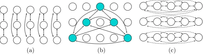
Next, we consider Hopf bifurcation based onV₃−. This bifurcation is driven by Hopf bifurcation of S4 on V3, which has been analyzed in [27]. (The stability of resulting solutions is discussed on p. 634 in [31].) Up to conjugacy, these authors find five typesΣ1, . . . , Σ5 of periodic solutions whose structures are listed in Ta-ble1. Patterns corresponding toΣ1give rivalry between the derived patterns shown in Fig.10(a) (note that because of symmetry, Figs.10(b) and10(c) are conjugate to Fig.10(a), and all three patterns coexist). Patterns corresponding toΣ3are those shown in Fig.11; patterns corresponding toΣ5are those shown in Fig.12. We have not computed the transition of patterns that are associated withΣ4solutions.

We have focused on the simplified version of the conventionalcolored dot experi-ment with a 2×2 grid of dots. However, the bifurcations using a 6×4 grid of dots, as in the original experiment [2], are completely analogous. Suppose there arendots.

Fig. 10 Predicted percept alternations for proposed conventionalcolored dotexperiment. Rivalry between

Fig. 11 Predicted percept alternations for proposed conventionalcolored dotexperiment. Rivalry in a rotating wave

Fig. 12 Predicted percept alternations for proposed conventionalcolored dot

experiment. Rivalry between

three dots of one color

Then there will benattribute columns with a symmetry groupΓ =Sn×Z2(ρ). The

isotypic decomposition is

V1=

(X, . . . , X):X∈R2

Vn−1=

(X1, . . . , Xn):Xj∈R2;X1+ · · · +Xn=0

It follows that the irreducible representations ofΓ acting onR2n_=Rn_⊕Rn_are

V₁+=(v, v):v∈V1

fusion

V₁−=(v,−v):v∈V1

learned: single color

V_n+₋₁=(v, v):v∈Vn−1

fusion

V_n−₋₁=(v,−v):v∈Vn−1

derived: scrambled colors

(7)

Hence, the bifurcation structure forndots is analogous to that of 4 dots; there are two types of bifurcation to fusion states (V_n+₋₁,V₁+), one to rivalry between the learned patterns (V₁−), and one to bifurcation to derived patterns (V_n−₋₁). The actual solution types depend onnand we will not attempt to interpret the bifurcation results of [27] in thendot case as we have in the four dot case.

3.3 The ScrambledColored DotNetwork

is one of several types of possible solutions and it is not clear why this particular solution type should be observed for such a large percentage of the time.

If, however, we include lateral coupling we arrive at the network in Fig.9whose symmetry group isΓ =D4×Z2(ρ). Differential equations that correspond to this network have the form

˙

X1=f (X1;X2;X3,X5,X7;X4,X5,X8) ˙

X2=f (X2;X1;X4,X6,X8;X3,X6,X7) ˙

X3=f (X3;X4;X1,X5,X7;X2,X6,X7)

˙

X4=f (X4;X3;X2,X6,X8;X1,X5,X8)

˙

X5=f (X5;X6;X1,X3,X7;X1,X4,X8) ˙

X6=f (X6;X5;X2,X4,X8;X2,X3,X7) ˙

X7=f (X7;X8;X1,X3,X5;X2,X3,X6)

˙

X8=f (X8;X7;X2,X4,X6;X1,X4,X5)

(8)

where the overbar indicates terms whose order can be interchanged. The form of (8) emphasizes the fact that there are three different types of coupling: inhibitory, excitatory learned, and excitatory lateral.

The isotypic decomposition ofR8 _{underΓ =D4×Z2(ρ)now has six} compo-nents, as follows. Let

W0=

(X, X, X, X):X∈R2

W1=

(X,−X, X,−X):X∈R2

W2=

(X1, X2,−X1,−X2):X1, X2∈R2

It follows that the isotypic components ofΓ acting onR16=R8⊕R8are

W₀+=(v, v):v∈W0

fusion

W₁+=(v, v):v∈W1

fusion

W₂+=(v, v):v∈W2

fusion

W₀−=(v,−v):v∈W0

learned: scrambled color

W₁−=(v,−v):v∈W1

derived: single color

W₂−=(v,−v):v∈W2

derived: other scrambled colors

(9)

abstract point of view, the Wilson network with lateral coupling is a much more satisfactory explanation for the existence of the single color rivalry when scrambled dots are presented than is the Wilson network without lateral coupling.

Finally, we note that the discussion in this section generalizes to the scrambled dot experiment with a 6×4 grid of colored dots, as long as the number of green dots and the number of red dots in the scrambled learned patterns are equal, as in Fig.4(b).

4 Stability in ScrambledMonkey-TextNetworks

The classification of possible solution types, as given in Sect.3, is model independent. We do not need to know the particular equations in order to complete the classifica-tion; we just need to know that the equations areΓ-equivariant. Given a system of equations, we can prove that solutions of the types that we have classified actually exist only by showing that a Hopf bifurcation that corresponds to the appropriate isotypic component actually occurs. See the equivariant Hopf theorem in [5]. We can also determine whether these solutions are stable, which is model dependent; we need to know the equations.

There are three steps in the calculation of stability. First, we need to determine that there is a fusion equilibrium. Second, we must show that the Hopf bifurcations them-selves can be stable. That is, we must find Hopf bifurcation points where the critical eigenvectors of the JacobianJ at the fusion equilibium correspond to the given iso-typic component and all other eigenvalues ofJhave negative real part. Third, we need to calculate higher order terms in a center manifold reduction to check that the bifur-cating solutions are actually stable. Alternatively, we can just simulate the equations for parameter values near a stable Hopf point and see whether we can detect stable so-lutions. Indeed, this was our approach for the scrambledmonkey-textmodel in Sect.2. The principal conclusion is that derived pattern rivalry (between unscrambled im-ages) can be stable in this model only if the strength of the lateral coupling is greater than the strength of the learned pattern coupling (see Proposition3). Note that this cannot happen if lateral coupling is absent. We also show that learned pattern rivalry (between scrambled images) can only be stable when the strength of the learned pat-tern coupling is greater than the strength of the lateral coupling (see Proposition2).

4.1 Equations for the ScrambledMonkey-TextNetwork

There is some leeway in choosing differential equations associated to a given net-work. In this context, we follow Wilson and others and assume that the nodes are neurons or groups of neurons and that the important information is captured by the firing rate of the neurons. Thus, we follow [1] and assume that in these models each node(i, j )in the network has a state spacexij=(x_ijE, x_ijH), wherex_ijE is an

activ-ity variable (representing firing rate) andx_ijH is a fatigue variable. Coupling between nodes is given through a gain functionG. Specifically,

εx˙_ijE= −x_ijE+G

Iij+w

pq→ij

x_pqE +δ

uv→ij

x_uvE −β

rj⇒ij

x_rjE−gx_ijH

˙

x_ijH=x_ijE−x_ijH

where→indicates an excitatory learned pattern connection,→indicates an excita-tory lateral connection, and⇒indicates an inhibitory connection. Similar rate models are often used in the rivalry literature (Wilson et al. [32,33]). The parameters are: re-ciprocal learned pattern excitation between nodesw >0, reciprocal lateral excitation

δ≥0, reciprocal inhibition between nodesβ >0, the external signal strengthIij≥0

to nodes, the strength of reduction of the activity variable by the fatigue variable

g >0, and the ratio of time scalesε <1 on which∗Eand∗H evolve. Note thatδ=0 for the simulations in [1]. The gain functionGis usually assumed to be nonnegative and nondecreasing, and is often a sigmoid.

In this case, we assume allIij=I and for the network in Fig.6(c) the system (10)

reduces to:

εx˙₁₁E = −x₁₁E +GI+wx₂₂E +δx₁₂E −βxE₂₁−gx₁₁H ˙

x₁₁H=xE₁₁−x₁₁H

εx˙₂₁E = −x₂₁E +GI+wx₁₂E +δx₂₂E −βxE₁₁−gx₂₁H ˙

x₂₁H=xE₂₁−x₂₁H

εx˙₁₂E = −x₁₂E +GI+wx₂₁E +δx₁₁E −βxE₂₂−gx₁₂H ˙

x₁₂H=xE₁₂−x₁₂H

εx˙₂₂E = −x₂₂E +GI+wx₁₁E +δx₂₁E −βxE₁₂−gx₂₂H ˙

x₂₂H=xE₂₂−x₂₂H

(11)

As we will see, there is an advantage of lateral coupling in the four-node model for the scrambledmonkey-textexperiment. The additional coupling allows the rivalrous solutions with respect to the derived patterns to be asymptotically stable at bifurca-tion; these solutions are not stable if lateral coupling is excluded.

4.2 Calculation of Fusion Equilibria

The equations for a fusion equilibrium for (11) reduces to

x=GI+(w+δ−β−g)x (12)

where allx_ijE=x_ijH=x. Solutions of this equation have been studied by [10,11,34]. It is convenient to define

ρ=w+δ−β−g

Then (12) can be rephrased as

G(I+ρx)−x=0 (13)

Diekman et al. (Lemma 3.1 in [34]) state that for everyρthere is anI >0 andx >0 that satisfies (13). Thus, we can assume there is a fusion state for any choice ofw,δ,

Lemma 1 Fixw, δ, β, g, I, G₀>0.Fixx0>0so that the(I−x0)ρ >0.Then there exists a gain functionG(z)satisfying

G(x0)= 1

ρ(x0−I ) (14)

andG(z0)=G₀.

It follows from Lemma1thatx0is a fusion equilibrium and that we can choose G_{(x0) >0 arbitrarily.}

Proof of Lemma1 The sigmoidal function

G(x)= 2a

1+e−(2b/a)(x−x0)

satisfiesG(x0)=a andG(x0)=b. Setb=G₀>0 anda equal to the RHS of (14), which is also positive sinceρandx0−I have the same sign. 4.3 Calculation of Critical Eigenvalues

J++=

−1+(w+δ−β)G −gG

ε −ε

J+−=

−1+(−w−δ−β)G −gG

ε −ε

J−+=

−1+(−w+δ+β)G −gG

ε −ε

J−−=

−1+(w−δ+β)G −gG

ε −ε

(15)

detJ++=ε1+(g+β−w−δ)G

detJ+−=ε1+(g+β+w+δ)G

detJ−+=ε1+(g−β+w−δ)G

detJ−−=ε1+(g−β−w+δ)G

(16)

trJ++= −1+(w+δ−β)G−ε

trJ+−= −1+(−w−δ−β)G−ε

trJ−+= −1+(−w+δ+β)G−ε

trJ−−= −1+(w−δ+β)G−ε

(17)

4.4 Stability of Learned Pattern Rivalry

Proposition 2 To have stable Hopf bifurcation to learned pattern rivalry in(11),it is necessary that

β > δ

w > δ (18)

Sufficient conditions for stable Hopf bifurcation to learned pattern rivalry are given by(18)and

g > w−δ+β

G> 1 w−δ+β

(19)

Proof For Hopf bifurcation to learned pattern rivalry to exist, we need tr(J−−)=0, that is,

ε= −1+(w−δ+β)G

It follows from (19) thatε >0. For this bifurcation to be stable we also need the other three traces to be negative. Thus, substituting forεin (17), we obtain the necessary conditions

trJ++<0 β > δ

trJ+−<0 β+w >0

trJ−+<0 w > δ

(20)

Note that the necessary conditions (18) follow from directly from (20) and the second condition in (20) follows from the first and third.

To prove the sufficiency part of the lemma, we need to verify that the determinants are all positive. This follows from (16) if

g+β−w−δ >0

g+β+w+δ >0

g−β+w−δ >0

g−β−w+δ >0

(21)

Note that the second inequality is always satisfied and, assuming (18), the first and third follow from the fourth. Finally, the fourth inequality follows from (19).

4.5 Stability of Derived Pattern Rivalry

Proposition 3 To have stable Hopf bifurcation to learned pattern rivalry in(11),it is necessary that

β > w

δ > w (22)

Sufficient conditions for stable Hopf bifurcation to learned pattern rivalry are given by(22)and

g > δ−w+β

G> 1 δ−w+β

(23)

Proof For Hopf bifurcation to derived pattern rivalry, we need tr(J−+)=0, that is,

ε= −1+(−w+δ+β)G

It follows from (23) thatε >0. For this bifurcation to be stable, we need the other three traces to be negative. On substituting forε in (17), we obtain the necessary conditions:

trJ++<0 β > w

trJ+−<0 β+δ >0

trJ−−<0 δ > w

(24)

Note that the necessary conditions (22) follow directly from (24) and the second condition in (24) follows from the first and third.

To prove the sufficiency part of the lemma, we need to verify that the determinants are all positive. This follows from (16) if the four conditions (21) are satisfied. Note that the second inequality is always satisfied and, assuming (22), the first and fourth follow from the third. Finally, the third inequality follows from (23).

Note that Hopf bifurcation to stable derived patterns is possible only when the strength of the lateral coupling is larger than the strength of the learned pattern cou-pling; that is,δ > w.

5 Discussion

We have shown that the surprising results in three binocular rivalry experiments de-scribed by Kovács et al. [2] can be understood through the use of Wilson-type net-works [1] and equivariant Hopf bifurcation theory [5], as interpreted in coupled cell systems [3].

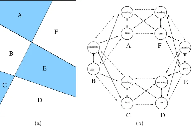
Fig. 13 aRegions A–Finimage rectangleof scrambledmonkey-textexperiment.bNetwork withsix attribute columnscorresponding to monkey or text image in each region. All inhibitory couplings are shown, but only “nearest neighbor” learned and lateral couplings are shown

reduction uses the notion of a quotient network discussed in [3] and proceeds by identifying equivalent levels in different attribute columns. LetSdenote the subspace obtained in this way [34]. This subspace is flow-invariant for the dynamics; moreover, if one uses the rate models (10) (without lateral coupling), then there are regions in parameter space where the dynamics are attracting toS. We mention this for two reasons. First, bifurcation in directions transverse to S yields the derived patterns discussed in this paper. For such bifurcations to occur,Scannot be attracting and this occurs when lateral coupling is present. Second, one can think of the reduction toS (that is, reduction to the two-node network) as aggregating the information contained in several different attributes into one combined attribute. We believe this is a more general phenomenon with different levels of pattern complexity, as we now describe. To construct a Wilson network for a given experiment, we must assume which attributes and which levels appropriately define a pattern. For example, in the sim-plifiedcolored dotexperiments, we assume that the attributes are the colors of the dots at four geometric locations. On the other hand, in the scrambled monkey-text experiment, we assume that the attributes are the kind of picture (monkey or text) in two regions of the image rectangle (the blue and the white regions in Fig.6(a)). One can ask whether these attributes are the reasonable ones to describe patterns in these experiments.

dotexperiments. It is reasonable to ask whether there is a relationship between the networks in Figs.6(c) and13(b), and there is. The larger network in Fig.13(b) has a quotient network on the flow-invariant subspace

Fix(ACE)(BDF)= {XiA=XiC=XiE andXiB=XiD=XiF fori=1,2}

(see [3]) that is isomorphic to the smaller network in Fig.6(c). Hence, the solution types that we discussed previously for the smaller network also appear in the larger network (which corresponds to a more refined geometry). In principle, other solu-tion types can appear in the larger network, but there were no indicasolu-tions of such solutions in the scrambledmonkey-text experiment. We believe that there is a gen-eral relationship between refined patterns (the addition of extra attribute columns in Wilson networks) and the quotient networks from coupled cell theory [3].

There are two prevalent views about what leads to alternations during binocular rivalry:eye-basedtheories postulate that the two eyes compete for dominance, while stimulus-basedtheories postulate that it is coherent perceptual representations that are in competition (Papathomas et al. [24]). Kovács et al. [2] interpreted their results on interocular grouping (IOG) as evidence against eye-based theories of rivalry.

Lee and Blake [21] reexamine IOG during rivalry, and argue that, whereas IOG rules out models of rivalry in which one eye or the other is completely dominant at any given moment, IOG can be explained by simultaneous dominance of local eye-based regions distributed between the eyes. To demonstrate this, they performed a series of experiments using the Kovácsmonkey-textimages and an eye-swap tech-nique that exchanges rival images immediately after one becomes dominant (Blake et al. [35]). In their analysis, [21] consider a decomposition of themonkey-text im-ages into six regions that is very similar to the decomposition shown in Fig.13(a). Our mathematical construction, based on Wilson networks and an abstract notion of quotient networks, is not meant to represent V1 or any specific brain area. However, our results support the conclusion of [21] that global IOG (derived patterns) can be achieved by simultaneous local eye dominance.

We end by noting that it should be possible to test our predictions of likely per-cepts by performing the simplifiedcolored dotexperiments. We also note that illu-sions are part of this network theory and they themselves can lead to interesting kinds of perceptual alternations. This topic, as well as symmetry-breaking steady-state bi-furcations that lead to various types of winner-take-all states, will be discussed in future work.

Competing Interests

The authors declare that they have no competing interests.

Authors’ Contributions

Acknowledgements The authors thank Randolph Blake, Tyler McMillen, Jon Rubin, Ian Stewart, and Hugh Wilson for helpful discussions. YW thanks the Computational and Applied Mathematics Department of Rice University for its support. This research was supported in part by NSF Grant DMS-1008412 to MG and NSF Grant DMS-0931642 to the Mathematical Biosciences Institute.

References

1. Wilson HR:Requirements for conscious visual processing. InCortical Mechanisms of Vision. Edited by Jenkins M, Harris L. Cambridge: Cambridge University Press; 2009:399-417.

2. Kovács I, Papathomas TV, Yang M, Fehér A:When the brain changes its mind: interocular group-ing durgroup-ing binocular rivalry.Proc Natl Acad Sci USA1996,93:15508-15511.

3. Golubitsky M, Stewart I:Nonlinear dynamics of networks: the groupoid formalism.Bull Am Math Soc2006,43:305-364.

4. Golubitsky M, Stewart I:The Symmetry Perspective: From Equilibrium to Chaos in Phase Space and Physical Space. Basel: Birkhäuser; 2002.

5. Golubitsky M, Stewart I, Schaeffer DG:Singularities and Groups in Bifurcation Theory: Volume II. New York: Springer; 1988. [Applied Mathematical Sciences, vol 69.]

6. Blake R, Logothetis NK:Visual competition.Nat Rev, Neurosci2002,3:1-11. 7. Your amazing brain[http://www.youramazingbrain.org/supersenses/necker.htm]

8. Laing CR, Frewen T, Kevrekidis IG:Reduced models for binocular rivalry.J Comput Neurosci

2010,28:459-476.

9. Moreno-Bote R, Rinzel J, Rubin N:Noise-induced alternations in an attractor network model of perceptual bistability.J Neurophysiol2007,98:1125-1139.

10. Curtu R:Singular Hopf bifurcations and mixed-mode oscillations in a two-cell inhibitory neural network.Physica D2010,239:504-514.

11. Curtu R, Shpiro A, Rubin N, Rinzel J:Mechanisms for frequency control in neuronal competition models.SIAM J Appl Dyn Syst2008,7:609-649.

12. Kalarickal GJ, Marshall JA:Neural model of temporal and stochastic properties of binocular rivalry.Neurocomputing2000,32:843-853.

13. Laing C, Chow C:A spiking neuron model for binocular rivalry.J Comput Neurosci2002,12 :39-53.

14. Lehky SR:An astable multivibrator model of binocular rivalry.Perception1988,17:215-228. 15. Matsuoka K:The dynamic model of binocular rivalry.Biol Cybern1984,49:201-208. 16. Mueller TJ:A physiological model of binocular rivalry.Vis Neurosci1990,4:63-73.

17. Noest AJ, van Ee R, Nijs MM, van Wezel RJA:Percept-choice sequences driven by interrupted ambiguous stimuli: a low-level neural model.J Vis2007,7(8):10.

18. Seely J, Chow CC:The role of mutual inhibition in binocular rivalry.J Neurophysiol 2011,

106:2136-2150.

19. Liu L, Tyler CW, Schor CM:Failure of rivalry at low contrast: evidence of a suprathreshold binocular summation process.Vis Res1992,32:1471-1479.

20. Shpiro A, Curtu R, Rinzel J, Rubin N:Dynamical characteristics common to neuronal competition models.J Neurophysiol2007,97:462-473.

21. Lee S, Blake R:A fresh look at interocular grouping during binocular rivalry.Vis Res2004,

44:983-991.

22. Diaz-Caneja E:Sur l’alternance binoculaire.Ann Ocul1928,October:721-731.

23. Alais D, O’Shea RP, Mesana-Alais C, Wilson IG:On binocular alternation. Perception2000,

29:1437-1445.

24. Papathomas TV, Kovács I, Conway T:Interocular grouping in binocular rivalry: basic attributes and combinations. In Binocular Rivalry. Edited by Alais D, Blake R. Cambridge: MIT Press; 2005:155-168.

25. Tong F, Meng M, Blake R:Neural bases of binocular rivalry.Trends Cogn Sci2006,10:502-511. 26. Bressloff PC, Cowan JD, Golubitsky M, Thomas PJ, Wiener MC:Geometric visual hallucinations,

Euclidean symmetry, and the functional architecture of striate cortex.Philos Trans R Soc Lond B, Biol Sci2001,356:299-330.

28. Wilson H:Minimal physiological conditions for binocular rivalry and rivalry memory.Vis Res

2007,47:2741-2750.

29. Blasdel GG:Orientation selectivity, preference, and continuity in monkey striate cortex.J Neu-rosci1992,12:3139-3161.

30. Golubitsky M, Shiau L-J, Torok A:Bifurcation on the visual cortex with weakly anisotropic lateral coupling.SIAM J Appl Dyn Syst2003,2:97-143.

31. Dias APS, Rodrigues A:Hopf bifurcation with SN-symmetry.Nonlinearity2009,22:627-666. 32. Wilson H:Computational evidence for a rivalry hierarchy in vision.Proc Natl Acad Sci USA2003,

100:14499-14503.

33. Wilson H, Blake R, Lee S:Dynamics of traveling waves in visual perception.Nature2001,412 :907-910.

34. Diekman C, Golubitsky M, McMillen T, Wang Y:Reduction and dynamics of a generalized rivalry network with two learned patterns.SIAM J Appl Dyn Syst2012,11:1270-1309.

35. Blake R, Yu K, Lokey M, Norman H:What is suppressed during binocular rivalry?Perception