J Wood Sci (1998) 44:337-342 © The Japan Wood Research Society 1998
T o s h i r o T o c h i g i • C h i a k i T a d o k o r o • J u n K o b a y a s h i I z u m i S u g a w a r a • S a c h i e T a k a h a s h i
Improving production systems of timber-processing plants IV:
Application of genetic algorithms for appropriate positioning
of processing machines
Received: November 14, 1997 / Accepted: April 22, 1998
A b s t r a c t The development of a layout plan for a new plant with the aid of genetic algorithms was studied to place the machines so that the plant floor was effectively utilized and the operation would not be impeded. Genetic algorithms are search algorithms based on the mechanics of natural evolution and natural genetics to solve problems in engi- neering fields. Simulation with the aid of genetic algorithms was undertaken step by step. The first seven hundred strings (chromosomes) were generated at random to organize an initial population. Each string consisted of 40 bits (genes), which represented characteristics of machines (x- and y-coordinates and inlet and outlet formations of materials on machines) in the binary coding. Then the simulation was undertaken by repeating selection, cross- over, reproduction, and mutation of strings until all strings were saturated with the highest evaluation (fitness of chro- mosomes to environments in the case of creatures). Under some limitations, an acceptable layout plan of the modeled plant involving four wood-processing machines was ob- tained according to evaluation indices.
K e y w o r d s Genetic algorithms • Plant design • Production control
Introduction
As when constructing a new plant on a limited site or reestablishing the processing system of an existing plant so T. Tochigi ( ~ ) . C. Tadokoro
Institute of Agricultural and Forest Engineering, University of Tsukuba, Tsukuba, 305-8572, Japan
Tel. + 81-298-53-4894; Fax +81-298-53-4894 e-mail: [email protected] J. Kobayashi. I. Sugawara • S. Takahashi
Faculty of Regional Environment Science, Tokyo University of Agriculture, Tokyo 156-8502, Japan
Part III of this series appeared in Mokuzai Gakkaishi 37: 702~10, 1991. Part of this report was presented at the 47 th annual meeting of the Japan Wood Research Society, Kochi, April 1997
it can produce new products, if the structure and floor area of the plant are already specified we must determine the most appropriate place to locate the processing machines. Another consideration is the most suitable transportation route between these machines. In past studies, after discuss- ing the P E R T method, the queuing theory, the O R tech- nique, and the network theory, we introduced a computer simulation based on a calculus-based method (random search algorithms). 1'2 Unfortunately, it required a huge amount of time and labor. In this study we introduce genetic algorithms to solve the optimum layout problem mentioned above.
Evolution of creatures and genetic algorithms
Evolution of creatures and exchange of genes
From the formation of the earth to the present, environ- mental conditions have been changing dramatically. During the development of the earth millions of plant and animal species have appeared, and large numbers have disap- peared. Only those that adapted to their environment have survived and continued their evolution. Biological evolution entails repeated genetic changes, and the proce- dure can be defined simply as follows: (1) crossover; (2) reproduction; (3) selection; and (4)Mutation.
Crossover is the partial exchange of genetic materials
(mainly genes) between homologous chromosomes (par- ents) by their mating. It yields two new chromosomes (children) partially with their parents' chromosomes.
Reproduction is the process by which individual chromo-
in a chromosome with low survival probability. Mutation rates are extremely low in nature.
Genetic algorithms
Genetic algorithms (GAs) are search algorithms based on the mechanics of natural evolution and natural genetics] '4 In every generation, a new set of artificial creatures (chro- mosomes, called "strings" in GAs) is created using "bits" (genes) and pieces of the fittest of the earlier generation. Therefore, GAs are defined as computer simulation techniques that can solve problems in engineering fields by artificially imitating the mechanics of natural evolution.
The mechanics of a simple G A are simple, involving nothing more complex than a rearrangement of strings in order (selection of chromosomes), copying strings
(reproduction of chromosomes), exchanging partial
strings (crossover of chromosomes), and occasional and random alteration of a bit (mutation of a gene).
Model plant
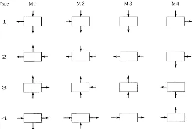
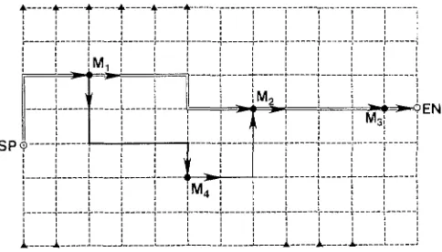
The floor area of a model plant is proposed hypothetically. It is limited and divided into 12 × 7 grids, as shown in Fig. 1. We assume that four processing machines must be placed on the floor, and their arrangements are defined as shown in Fig. 2. Inlet and outlet formations of materials on machines are defined as shown in Fig. 3. The nodes of the grids are places where processing machines could be placed.
Limitations for designing the model plant
To design a model plant, the following limitations are tentatively established.
1. Positional limitation. An entrance gate of raw materi-
als (SP, Fig. 1) and an output gate of products (EN, Fig. 1)
I, . . . i .. .... ... .. 1 . . .
' - . . . i . . . ~----<~ EN
', I I < I I I I I I I '~ I
, , , I i ; I I I i i I I
. . . ~ . . . ~ . . . L . . . • . . . j . . . L . . . ' . . . " . . . 2 - . . . L . . . ' . . . I
I I '
. . . l . . . r . . . r . . . ~ . . . I . . . F . . .
l
I i : I I I
, I
4 ... ' ... ~ ... L ... ,< ...
i ! i i i i ! i i i i i
I ; ~ i i ; I '. ', I I ',
i J i i , i i i a L i L
' l i I I I I ' l i I
. . . L . . . ', . . . i . . . L . . .
4 8 1 2
Fig. L Floor area of a model plant divided into 12 × 7 grids. SP,
entrance gate of raw materials; EN, output gate of products
Fig. 2. Proposed arrangements of processing machines in the model
plant. M1-M4, processing machines; ~ , main production line; >,
secondary production line from M 1 to M4; ---->, secondary production
line from M 4 to M 2. Arrows represent paths of material flow
T ~ e M l M 2 M 3 M 4
2
i
3
4
Fig. 3. Inlet and outlet formation of materials on machines processing machines
were fixed, and their coordinates were given by (1, 2) and (13, 7), respectively. Because of conditions of a plant's loca- tion and function, there are certain areas where machines and transportation routes cannot be installed.
2. Distance from machine to machine. The Distance
from the entrance gate of the raw materials (SP) to the first machine (M1), from M: to the second machine (M2),
from M2 to the third machine (M3) and from M1 to
the fourth machine (M4) w e r e defined as -> 4, 6, 4, and 5
units, respectively, even if materials were transported horizontally or vertically (or both). What is meant here by "a unit "is the distance between the node of the grid and the adjoining node (width of a grid).
3. Relation between machines. The x-coordinate of
M 4 should be more than that of Mt and less than that of
M2 simultaneously. The y-coordinate of M 4 should be less
than the y-coordinates of M1 and M2 simultaneously.
4. Transportation rate o f materials. It was possible to
change the direction of the route to the x- and y-axes only at the nodes of the grids. As the routes were installed to trans- port materials from one machine to others, the route could not be extended backward to prevent a counterflow of materials once the route had been extended. Overpassing the existing routes was also prohibited. The transportation rate of materials for running horizontally was defined and required 2 s/unit. Vertically it took 1 s/unit. Turning the run- ning direction, from horizontal to vertical or vice versa, consumed 0.5 s once.
Simulation of the layout plan by GA
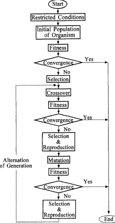
Procedures of the G A simulation
A simulation procedure of genetic algorithms to obtain the fittest layout of wood-processing plants was undertaken step by step as shown in Fig. 4: Seven hundreds of strings were generated at random, and they organized the initial population as shown in Fig. 5. Each string consisted of 40 bits. Therefore, this population was chosen through 28000 (700 × 40) successive randomization. In a string, each 10 bits were provided for representing characteristics of a machine in a binary coding. The x- and y-coordinates of a machine were represented by four bits each, two bits were used for the inlet and outlet formations on the machine, respectively.
Selection, the next step of the G A simulation, is a pro- cess wherein individual strings are rearranged according to their fitness (descrited later). Strings with higher fitness values were ranked in the upper portion of the population and had a higher probability of contributing one or more offspring to the next generation according to priorities of fitness determined by the weighted roulette method. 4 This operation was an artificial version of natural selection, a darwinian survival of the fittest among chromosome creatures.
Reproduction is an inevitable process that creates new strings to the next generation. In this study it was done in
339
Alternation
of Generation
[Restricted Conditions I
Initial Population I
of Organism [
~
YesICrossoverl
Yes
Se o tio" I
Reproductionl
~
YesSelection
Reproduction
J
Fig. 4. Flow of genetie algorithm (GA) simulation in this study
three ways, as shown in Fig. 6: The first step was an exact copying of the strings with high fitness values after the selection of strings in the old population, the second was transformation of strings in order of fitness, and the third was random transformation of strings from the old popula- tion to the new.
After reproduction of the strings to the new population, simple (one-point) crossovers of strings proceeded. 5 First, two strings were mated at random. After deciding on the position of bits (k) at random between 1 and string length less than 1 (L - 1), the paired strings underwent crossing- over by exchanging all bits between k + 1 and L, inclusively, as shown in Fig. 7; then two new strings were created from their parents. Because strings with higher fitness values were given higher priorities for crossing over, they crossed over many times and exchanged their strings with different mates at each crossover. In this study, strings for crossing over were decided at random according to their fitness values.
1 0 1 0 1 0 1 0 1 1 0 0 1 0 0 1 0 0 0 1 0 1 0 1 1 0 1 0 0 0 0 0 0 0 0 0 1 0 0 0 0 0 0 0 1 1 1 . 1 1 0 0 1 0 0 1 0 0 1 0 1 1 1 0 0 0 0 1 0 1 1 0 1 0 1 0 0 1 0 1 0 1 1 0 1 0 1 0 1 0 0 0 1 0 1 1 0 0 1 0 0 0 1 1 1 0 1 0 1 0 0 0 1 0 0 1 1 1 0 1 0 1 1 1 1 0 1 1 0 0 0 0 1 1 0 0 0 0 1 0 0 1 1 1 1 0 1 0 1 0 0 1 1 0 1 0 1 1 1 1 0 0 1 1 0 0 0 1 0 0 1 0 0 1 0 0 1 1 1 0 1 . 1 0 0 1 0 0 0 1 1 0 1 1 0 1 0 0 0 0 0 0 0 0 0 1 0 1 1 1 0 1 1 1 1 1 1 1 0 0 0 1 1 0 1 1 0 0 0 1 1 0 0 0 0 0 0 0 1 1 1 1 0 1 1 1 0 1 1 0 1 1 0 1 1 1 1 0 1 0 1 0 1 0 0 1 0 1 1 1 1 1 1 0 1 0 0 0 1 0 0 0 1 0 1 0 1 0 1 1 0 1 1 1 1 0 0 0 1 1 1 0 0 0 1 0 0 0 0 1 1 1 0 0 0 0 1 0 1 0 1 0 1 1 0 1 0 1 1 1 0 1 1 0 1 1 0 1 0 1 1 0 1 0 0 1 1 1 0 0 1 1 1 0 1 0 0 1 1 1 1 0 0 0 0 1 1 i l l 0 0 1 0 0 1 0 0 1 1 1 0 0 1 1 1 1 0 1 0 1 0 0 0 0 1 1 1 0 0 0 1 0 0 0 0 0 0 0 0 1 0 0 1 0 0 1 0 0 1 1 0 0 1 1 0 0 0 0 0 1 0 0 1 1 0 0 0 0 1 0 0 0 0 1 1 1 0 0 1 1 1 1 1 1 0 0 0 1 0 0 1 0 0 0 1 1 0 0 0 0 1 0 1 1 1 1 0 1 0 1 0 0 I i 1 0 1 1 1 1 0 1 0 0 0 1 0 0 1 0 0 0 1 1 0 0 1 0 1 0 1 1 0 1 1 1 0 0 1 0 0 0 i l l l t 0 0 1 1 0 0 0 1 1 1 0 0 1 1 1 0 1 1 0 0 0 0 1 1 1 1 1 0 1 0 0 1 1 0 1 1 0 0 0 0 0 i i l 1 0 1 1 0 1 0 1 0 0 1 0 1 1 0 0 1 1 0 1 1 1 0 1 0 1 0 0 0 1 i l l l 0 1 1 0 1 i i 0 0 0 0 0 0 1 0 1 i I 1 0 0 0 1 1 0 1 1 0 0 0 1 1 0 1 1 0 i 0 0 0 0 0 i i 1 0 0 1 0 0 0 1 1 0 0 0 1 0 1 0 1 1 1 1 1 0 1 1 0 0 0 1 0 1 0 1 0 1 1 0 1 1 0 1 0 0 0 0 0 1 1 0 1 1 1 1 0 1 0 0 0 1 . 0 0 0 0 0 1 1 0 1 0 1 0 1 1 1 0 1 1 0 0 1 1 1 1 0 0 0 1 0 1 1 0 0 0 1 1 1 0 1 1 1 0 1 0 0 0 0 0 0 0 1 0 1 1 i l i 1 0 1 0 1 0 0 0 1 1 1 0 1 0 0 0 0 0 1 0 0 1 0 0 1 0 0 1 0 I i 1 0 0 1 0 1 1 0 1 0 1 0 1 0 1 1 1 1 1 0 1 1 0 0 1 0 1 1 0 0 1 1 1 0 1 0 0 1 1 0 0 1 0 0 1 1 1 0 1 1 1 1 1 1 0 0 1 0 1 1 1 0 1 0 0 1 1 1 0 0 0 1 1 0 1 0 0 1 1 1 1 0 0 0 0 1 0 0 1 1 0 1 0 0 0 1 1 0 1 1 1 0 1 1 0 0 1 1 1 0 1 1 1 0 1 1 0 1 0 0 0 1 1 0 0 1 1 1 1 1 0 1 0 0 1 1 0 0 0 0 1 1 1 1 1 1 0 1 0 0 0 1 0 0 0 1 0 1 1 1 1 0 0 1 1 1 1 0 1 1 1 1 0 1 1 0 1 1 0 0 1 1 0 0 1 1 0 0 1 0 0 1 0 1 0 0 1 1 0 1 1 1 0 1 1 1 1 0 1 1 1 1 0 1 I I 0 0 0 1 0 1 1 1 1 0 0 1 0 1 0 1 0 1 0 0 0 1 1 1 0 1 1 1 1 0 0 0 1 0 1 1 0 1 0 0 1 0 0 0 0 1 1 0 1 1 1 0 0 1 1 1 0 0 t 0 1 1 0 0 0 1 1 0 0 1 0 1 0 0 1 1 1 1 1 1 0 0 0 1 I I 0 0 0 1 0 1 1 1 1 0 0 1 1 1 1 0 0 0 1 1 1 0 1 1 0 0 0 0 0 0 0 1 1 0 1 1 0 1 1 0 1 0 1 0 0 0 0 1 0 1 1 0 1 0 1 1 0 0 0 1 0 1 0 1 1 0 0 1 1 1 0 1 0 0 i l l 0 1 1 0 1 0 0 1 1 0 1 0 1 1 1 0 1 0 0 0 1 0 0 1 0 1 0 0 0 0 1 0 1 0 1 1 1 1 0 1 0 0 0 0 0 0 0 1 1 0 0 0 1 0 0 1 0 0 1 1 1 0 0 1 0 1 1 0 0 1 0 0 1 1 0 1 0 0 0 I I 1 1 0 1 1 0 1 1 0 0 0 1 1 1 1 0 1 1 1 0 1 1 0 0 0 0 i 1 1 1 1 0 0 0 1 0 0 1 0 1 1 0 0 0 1 0 0 0 0 0 1 1 0 0 1 1 0 1 1 0 1 1 1 1 1 0 1 1 1 1 0 0 1 1 0 0 0 0 0 0 0 0 1 1 0 0 1 0 1 1 0 1 1 i l t 0 0 0 1 1 0 0 0 1 0 0 0 0 0 0 0 0 1 1 0 0 0 1 0 0 1 0 1 0 1 1 0 0 1 1 0 0 0 1 0 1 1 0 1 0 1 1 0 0 1 0 1 0 0 1 0 1 1 1 0 1 1 0 0 0 0 0 0 0 1 0 0 1 1 0 1 0 1 1 1 1 1 1 0 1 1 0 1 1 0 0 1 0 1 0 0 1 0 1 0 1 1 0 0 0 0 0 0 1 0 1 1 0 1 0 0 1 1 1 0 0 1 0 0 0 1 0 0 1 1
Fig. 5. Example of the initial population of creatures (strings) in the G A simulation
Strings(chromosomes)
:
Strings(chromosomes)
i
[ l lili lilii I" I' I I
Fig. 7. Simple (one-point) crossover of strings
String(chromosome)
Reproduction Fig. 8. Mutation of bits (genes) in a string
Population of organism
Fig. 6. Reproduction of strings introduced in this study. A, strings selected, in order of fitness; B, strings selected in random; C, copied strings
the population. The times of mutation were decided at random according to the frequency of mutations. When mutation occurred, a string and a bit were also decided at random, and the value of the bit was altered automatically. Simulation was undertaken until all of the strings in the population were saturated with the fitness value 6. When the simulation was completed, an optimum route for a line from
one machine to another was determined by the Dijkstra method, 7 which could determine the shortest route between two machines, avoiding crossing the existing routes.
Evaluation of the simulation (fitness)
During the course of manufacturing a product, there are various positions for the machines and routes connecting them to be considered. The best layout plan among such possibilities should be chosen with evaluation indices, called the "fitness value" in this study.
The speed of the processing machine was not considered in this study. Of course, a single condition or a combination of the following four conditions could be selected to deter- mine the most appropriate layout plan. In a natural popula- tion, fitness can be determined by the creatures' ability to survive predatory enemies and environments. In this study, simulated with respect to layout plans of wood-processing plants, to obtain the fittest conclusion fitness was evaluated by the following three indices and a supplemental one.
1. M i n i m u m distance. This step is to minimize the dis-
This does not mean that the time for transporting the mate- rials would be minimized as well. The length of an entire transportation route was obtained by summing the dis- tances between processing machines.
2. Minimum time consumption. The total time it took for
a material to pass over the entire route was determined. A comparison of routes was made by measuring the time needed for a material to enter the entrance gate of raw materials and reach the output gate of products, taking into consideration the distance between machines, and the time spent for transportation.
3. Minimum number of times for changing direction of
routes. To change the direction of a route too often would
result in complications for the layout plan and an instant impediment to the flow of materials, thereby taking m o r e time to transport materials. The total distance necessary for processing would mean greater construction costs. If the processing area exceeds the available space, however, it is necessary to change the direction of the route. In such a case, it would be best to install the fastest possible route and extend the parts of it that flow straight. O n the other hand, changing the direction of the route should shorten the slow portions of the route.
4. Comparison of area balance. This is a supplemental
index to evaluate the simulation. It considers the conditions pertaining to the balance within the space separated by transportation routes between the entrance gate of raw materials and the output gate of products.
Fitness values were obtained by summing the values of these three indices after each genetic action. Strings with smaller values were evaluated as having higher fitness. Evaluation with a supplemental index was also considered when the most advantageous string was determined.
Results and discussion
The ratios of fitness values to the final fitness (saturated) value for the whole population were calculated after each genetic action (Fig. 9). Simulation was started f r o m a hybrid population at first. As genetic actions were repeated and progressive generations were established, the fitness of the population changed to facilitate better survival. After about 50 generations, the population became homogeneous, consisting of close relatives. Afterward, if the renewal of generations was continued, the population returned to a hybrid one, and its ability to survive was becoming recessive.
After the whole-population saturated fitness value was determined, the final conclusion were drawn with respect to the r e c o m m e n d e d positions of machines, and their orienta- tion was obtained. The final output of the G A simulation is shown in Fig. 10. T h e r e c o m m e n d e d layout in the modeled wood-processing plant, the final result of the simulation, is shown in Fig. 11.
R e c o m m e n d e d layouts, when the entrance gate of raw materials and the output gate of products were changed, are illustrated in Figs.12-15.
0.8
~ 0 . 6
c-
~0.4
0.2
TTII
Ill,Ill
T
0
25
TTTtTTIITT'
l l l i i I iI TIT
II 7
Generation
50
7'5 16o
15o 17s
200
Fig. 9. Ratio of fitness values in the G A simulation. Vertical lines,
range of fitness values in the population ( m a x i m u m to minimum);filled
circles, ratio of s a t u r a t e d strings in the population
. . . Final Result
0 0 1 1 0 1 0 0 1 0 1 0 0 0 0 1 1 0 1 1 @
1 1 0 0 0 1 1 0 1 1 0 1 1 1 0 0 1 1 0 0
Ev(1) : 76.5 Q )
ICX= 3 ICY: 4
JCX= 8 JCY: 6
k32
MCX: 12 MCY~ 6
NCX= 7 NCY: 3
PTN$(1)= TYP3
PTN$(2) ~ TYP4 @
PTN$(3) = TYP4
PTN$(4)- TYP1
IK J K L D T EV X Y Q
36 S 1 4 1 6.5 11.5 2 2
1 2 7 1 12.5 20.5 5 2
2 3 4 0 8.0 12.0 4 0
3 E 2 1 3.5 6.5 1 1
1 4 5 1 9.5 15.5 4 1
4 2 4 1 5.5 10.5 l 3
01:04:53 26 5 45.5 76.5
Fig. 10. Final result of the G A simulation. Encircled Numbers: 1,
s a t u r a t e d string r e p r e s e n t e d its bits in binary coding; 2, fitness value of
the saturated string; 3, x- and y-coordinates of machines; 4, inlet and outlet formation of materials on machines; 5, data for the optimum layout plan representing generation (IK), total units from a machine or the input gate to a machine or the output gate (L), number of times to change the direction of a path (D), times required (T), fitness value
(EV) and horizontal and vertical units (X and Y) from a machine or the
input gate (J) to a machine or the output gate (K)
Conclusion
. . . . , ~ . . . . ~ . . . . . 4 , . . . ,'l"- . . . . ~ . . . r . . . ; . . . ] . . . ~ . . .
i
]
!
i
]
i
i
i
... ~ .. . . EN
' ' ' i 1 : I I
:
,:
,:
,'
i
iM2 i
,:
," ... i .... -I .... ? ... i ... i ... ~ 1 1 ... i ... i ... ~ ... i ... i
; ... ~ --M! > i ~ ... ; ... ,L ... ~ ... ~: ... i i { _~_ i i i ! ! i i i
i
'
il
. . .
SP L
• .... -i- .... J ... l ... ,'_ ... _, ... t ... ,k ... £ .... ~, ... i ... _,'
Fig. 11. Recommended layout plan in the modeled plant by the GA
simulation. Triangles, prohibited places to install processing machines
and transportation routes
• ... ~----e--"'-~ ... ~----* ... ; ... -~ ... c ... ~ ... ~ ... ; I I I I : : : : I
. . . ~- .. . . . i . . . f i . . . F . . . + . . . H
• ~ n n ~ ~ , ~ ~
_~ I lYl I I I I ; l
. . . ,. . . . 2 , ' - - - - 4 - . . . " . . . "
' '
.... '-;--11-
' ' '" . . . . k . . . 1 . . . ~ . . . . L L J
. . . . ~ n 1 : II , , ,
: I 1 , I : , , ,MR , ,
, I , - - - , L . . . k . . . 4 . . . , k - - - ~ . . . " ... -'
Fig. 14. Recommended layout plan when SP and EN were fixed on (1,5) and (13,4), respectively. See Fig. 11. for further explanations
: ' ' I . . . .
, : ', , ', I 1 I ~V , ~ I : ~ , : I ' 'IIAM. ~ ',: I
... i ... ~ ... ~: ... I- ... ~. ... i ... ] ... ~ ... ] ... - ~ - - - ~ ~ E N
. . . F . . . J . . . ~, .. . . ~" .. . . . T . . . ~, . . . F . . . ', . . . 1 . . . F . . . I
', I I I ', I I I ', I I
... J ... L ... L ... ~ ~ ~ _ LM~ - i_ ]
: ... r ... [ ... l ... r ... i
I ,i , 4, , ,
i i
! ... ! ... ,~ ... t ... ! ... ,~ ... t ... ! ... ~ ... ! ... ! ... ! ... !
" i " i i ! ! i " : : I : ~ . _ _ _ _ . j , . . . _L' . . . '.. . . -' . . . d . . . L . . . , L - - - A , - - - - - ~ i , . . .
Fig. 12. Recommended layout plan when SP and EN were fixed on (1,7) and (13,7), respectively. See Fig. 11 for further explanations
I I I I I
SP"i ... :!,, ... "I ... -I ... I- ... i,,, ... 4 ... :'i ... I" ... i=l ... :- ... I- ... ~,
' I i
I I I !
i i
: i
i
M3 I
. . . i . . . ~ . . . I- . . . -I . . . 4 - - i ' q l : ~ . . . i . . . ~ ( S E N
i ', ! i i i 4: : : : : : :
~ _ _ _ _ _ ~ . . . L . . . L . . . .' . . . - ' . . . . ~ _ _ _ _ . ~ . . . ~ - . . .
Fig. 15. Recommended layout plan when SP and EN were fixed on (1,7) and (13,2), respectively. See Fig. 11. for further explanations
i i t R l l i i i i i i
'
'
!! ! . ! '
. . .:
. . . . L , : . . . . . . ! . . . . . . . . .. . . ~ F N
. . . . . .
i
I
. . . . . . I . . . r i. . . . . . . . . . iJ : i J • - i • .__i . . . i . . . " . . . J
. . . ' , r ~ , - - ~ i E i L
i i K ~ i i K * I , , . . . , i . . i . . I t , i , i J ,
i i ; [ L [ i i
i i L i i i i i i t i i i
. . . ~ . . . r . . . r . . . 1 . . . ~ . . . i " . . . T . . . ~ . . . f . . . T . . . 1 . . . i
, L i i , J i
k _ _ _ _ ~, . . . " . . . J . . . L . . . J . . . " _ _ _ _ & . . . ~ _ _ - - ~ L . . . L . . .
Fig. 13. Recommended layout plant when SP and EN were fixed on (1,4) and (13,5), respectively. See Fig. 11. for further explanations
a b l e l a y o u t p l a n of t h e m o d e l p l a n t , i n v o l v i n g f o u r w o o d - p r o c e s s i n g m a c h i n e s . I n a f u t u r e study, t h e t i m e analysis of m a t e r i a l flows i n t h e w o o d - p r o c e s s i n g p l a n t s i m u l a t e d in this s t u d y will b e c o n s i d e r e d b y i n t r o d u c i n g t h e q u e u i n g theory.
W e b e l i e v e t h a t g e n e t i c a l g o r i t h m s are s t r o n g tools for solving p r o b l e m s i n e n g i n e e r i n g fields a n d o b t a i n i n g a n op- t i m u m s o l u t i o n if c a n d i d a t e s for t h e s o l u t i o n (strings in a n
initial p o p u l a t i o n ) a n d the final o p t i m u m s o l u t i o n c a n b e r e p r e s e n t e d in b i n a r y coding.
Acknowledgment The authors thank Dr. Koichi Ichihara, Associate
Professor, Institute of Agricultural and Forest Engineering, University of Tsukuba, for his valuable suggestions.
References
1. Tochigi T, Amemiya R, Tadokoro C, Hashimoto H (1988) Improving production systems of timber-processing plants. Part 1. Development of the computer-simulation procedure to design the production line, Mokuzai Gakkaishi 34:314-319
2. Tochigi T, Amemiya R, Tadokoro C, Hashimoto H (1988) Improving production systems of timber-processing plants. Part 2. Appropriate positioning of processing machines in sawmills. Mokuzai Gakkaishi 34:320-325
3. Holland JH (1992) Genetic algorithms. Sci Am 9:44-50
4. Goldberg DE (1989) Genetic algorithms in search, optimization, and machine learning. Addison-Wesley, New York, pp 10-18 5. Hirano H (1992) How to solve building-blocks problems by genetic
algorithms (in Japanese). Interface 2:108-112
6. Kitano H (1992) Genetic algorithms (in Japanese). Sangyo-Tosho, Tokyo, pp 13-14