R E S E A R C H
Open Access
Digital video stabilization based on
adaptive camera trajectory smoothing
Marcos R. Souza and Helio Pedrini
*Abstract
The development of multimedia equipments has allowed a significant growth in the production of videos through professional and amateur cameras, smartphones, and other mobile devices. Examples of applications involving video processing and analysis include surveillance and security, telemedicine, entertainment, teaching, and robotics. Video stabilization refers to the set of techniques required to detect and correct glitches or instabilities caused during the video acquisition process due to vibrations and undesired motion when handling the camera. In this work, we propose and evaluate a novel approach to video stabilization based on an adaptive Gaussian filter to smooth the camera trajectories. Experiments conducted on several video sequences demonstrate the effectiveness of the method, which generates videos with adequate trade-off between stabilization rate and amount of frame pixels. Our results were compared to YouTube’s state-of-the-art method, achieving competitive results.
Keywords: Video stabilization, Interest points, Trajectory smoothing, Video processing
1 Introduction
The availability of new digital technologies [1–8] and the reduction of equipment costs have facilitated the genera-tion of large volumes of videos in high resolugenera-tions. Several devices have allowed the acquisition and editing of videos, such as digital cameras, smartphones, and other mobile devices.
A large number of applications involve the use of digital videos such as telemedicine, advertising, entertainment, robotics, teaching, autonomous vehicles, surveillance, and security. Due to the large amount of video that are cap-tured, stored, and transmitted, it is fundamental to inves-tigate and develop efficient multimedia processing and analysis techniques for indexing, browsing, and retrieving video content [9–11].
Video stabilization [12–21] aims to correct camera motion oscillations that occur in the acquisition process, particularly when the cameras are mobile and handled by amateurs.
Several low-pass filters have been employed in the sta-bilization process [20,22]. However, their straightforward application using fixed intensity along all the videos is not suitable, since the camera motion may be unduly
*Correspondence:[email protected]
Institute of Computing, University of Campinas, Av. Albert Einstein 1251, Campinas 13083-852, Brazil
corrected when it should not. Recent approaches have used optimizations [23,24] to control the local smoothing intensity.
As a main contribution, this work presents and eval-uates a novel technique for video stabilization based on an adaptive Gaussian filter to smooth the camera trajec-tories. Experiments demonstrate the effectiveness of the method, which generates videos with proper stabiliza-tion rate while maintaining a reasonable amount of frame pixels.
The proposed method can be seen as an alternative to optimization approaches recently developed in the lit-erature [23, 24] with a lower computational cost. The results are compared to different versions of Gaussian filter, Kalman filter, and the video stabilization method employed in YouTube [24], which is considered a state-of-the-art approach.
This paper is organized as follows. Some relevant con-cepts and related work are briefly described in Section2. The proposed method for video stabilization is detailed in Section3. Experimental results are presented and dis-cussed in Section 4. Finally, some final remarks and directions for future work are included in Section5.
2 Background
Different categories of stabilization approaches [25–32] have been developed to improve the quality of videos, which can be broadly classified as mechanical stabiliza-tion, optical stabilizastabiliza-tion, and digital stabilization.
Mechanical stabilization typically uses sensors to detect camera shifts and compensate for undesired motion. A common way is to use gyroscopes to detect motion and send signals to motors connected to small wheels so that the camera can move in the opposite direction of motion. The camera is usually positioned on a tripod. Despite the efficiency usually obtained with this type of system, there are disadvantages in relation to the resources required, such as device weight and battery consumption.
Optical stabilization [33] is widely used in photographic cameras and consists of a mechanism to compensate for the angular and translational motion of the cameras, sta-bilizing the image before it is recorded on the sensor. A mechanism for optical stabilization introduces a gyro-scope to measure velocity differences at distinct instants in order to distinguish between normal and undesired motion. Other systems employ a set of lenses and sensors to detect angle and speed of motion for video stabilization. Digital stabilization of videos is implemented without the use of special devices. In general, undesired camera motion is estimated by comparing consecutive frames and applying a transform to the video sequence to compen-sate for motion. These techniques are typically slower when compared to optical techniques; however, they can achieve adequate results in terms of quality and speed, depending on the algorithms used.
Methods found in the literature for digitally stabiliz-ing videos are usually classified into two-dimensional (2D) or three-dimensional (3D) categories. Sequences of 2D transformations are employed in the first category to represent camera motion and stabilize the videos. Low-pass filters can be used to smooth the transformations, reducing the influence of high frequency of the camera [20,22]. In the second category, camera trajectories are reconstructed from 3D transformations [34,35], such as scaling, translation, and rotation.
Approaches that use 2D transformations focus on con-tributing to specific steps in their stabilization process [36]. By considering the estimation of camera motion, 2D methods can be further subdivided into two cate-gories [32]: (i) intensity-based approaches [37,38], which directly use the texture of the images as motion vector, and (ii) keypoint-based approaches [39,40], which locate a set of corresponding points in adjacent frames. Since keypoint-based approaches have a lower computational cost, they are most commonly used [22]. Techniques such as the extraction of regions of interest can be used in this step, in order to avoid cutting certain objects or regions that are supposed to be important to the observer [41].
Many methods have employed different motion fil-tering mechanisms, such as motion vector integration [39], Kalman filter [42, 43], particle filter [44], and reg-ularization [37]. Such mechanisms aim to remove high-frequency instability from camera motion [36]. Other approaches have focused on improving the quality of the videos, often lost in the stabilization process. The most commonly used techniques include inpainting to fill miss-ing frame parts [22,41,45], deconvolution to improve the video focus [22,41], and weighting of stabilization metrics and video quality aspects [36,45].
Recent improvements in 2D methods have made them comparable to 3D methods in terms of quality. For instance, the use of an L1-norm optimization can gener-ate a camera path that follows cinematographic rules in order to consider separately constant, linear, and parabolic motion [24]. A mesh-based model, in which multiple tra-jectories are calculated at different locations of the video, proved to be efficient in dealing with parallax without the use of 3D methods [23]. A semi-automatic 2D method, which requires assistance from the user, is proposed to adjust problematic frames [46].
On the other hand, 3D methods typically construct a three-dimensional model of the scene through structure-from-motion (SFM) techniques for smoothing motion [47], providing superior quality stabilization but at a higher computational cost [27, 47]. Since they usually have serious problems in handling large objects in the foreground [36], 2D methods are in general preferred in practice [36].
Although 3D methods can generate good results in static scenes using image-based rendering techniques [34, 48], they usually do not handle dynamic scenes correctly, causing motion blur [49]. Thus, the con-cept of content preservation was introduced, restrict-ing each output frame to be generated from a srestrict-ingle input frame [49]. Other approaches address this prob-lem through a geometric approximation by abdicating to be robust with respect to the parallax [35]. Other diffi-culties found in 3D methods appear in amateur videos, such as lack of parallax, zoom, and use of complemen-tary metal oxide semiconductor (CMOS) sensors, among others [47].
3 Adaptive video stabilization method
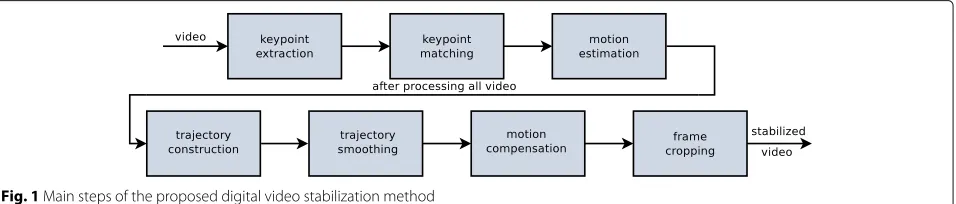
This section presents the proposed video stabilization method based on an adaptive Gaussian smoothing of the camera trajectories. Figure1 illustrates the main stages of the methodology, which are described in the following subsections.
3.1 Keypoint detection and matching
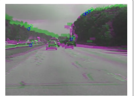
The process starts with the detection and description of keypoints in the video frames. In this step, we used the speeded up robust features (SURF) method [52]. After extracting the keypoints between two adjacent frames, their correspondence is performed using the brute-force method with cross-checking, where the Euclidean dis-tance between the feature vectors for each pair of points xi ∈ftandxj∈ ft+1is calculated for two adjacent frames ftandft+1. Thus,xicorresponds toxjif and only ifxiis the closest point toxjandxjthe closest toxi.
Figures 2 and 3 show the detection of keypoints in a frame and the correspondence between the points of two adjacent superimposed frames, respectively.
3.2 Motion estimation
After determining the matches between the keypoints, it is necessary to estimate the motion performed by the camera. For this, we estimate the similarity matrix, that is, the matrix that transforms the set of points in a frame ft to the set of points in a frame ft+1. Since
we consider the matrix of similarity, the parameters of the matrix transformation take into account camera shifts (translation), distortion (scaling), and undesirable motion (rotation) for the construction of a stabilization model.
In the process of digital video stabilization, oscillations of the camera that occurred at the time of recording must be compensated. The similarity matrix should take into account only the correspondences that are, in fact, between two equivalent points. In addition, it should not consider the movement of objects present in the scene.
The random sample consensus (RANSAC) method is applied to estimate a similarity matrix that considers only inliers in order to disregard the incorrect correspondences
and those that describe the movement of objects. In the application of this method, the value of the residual threshold parameter, which determines the maximum error for a match to be considered as inlier, is calcu-lated for each pair of frames. Algorithm 1 presents the calculation to determine the final similarity matrix.
Algorithm 1Similarity matrix computation 1: procedureFINALMATRIX
2: Generate the similarity matrixMby considering all matches.
3: Let MSE(M)be the mean square error of matrix M.
4: Apply the RANSAC considering the MSE(M)as residual threshold value.
5: Generate the similarity matrix M considering only the inliers obtained previously.
6: Let MSE(M)be the mean square error of matrix M.
7: Apply the RANSAC considering the MSE(M)as residual threshold value.
8: Generate the similarity matrixMfinalconsidering only the inliers obtained for the second execution of RANSAC.
In cases of pairs of frames with spatially variant motion, the correct matches also tend to have certain variation. Thus, the residual threshold is calculated so that its value is low enough to eliminate undesired matches and high enough such that the correct matches are maintained.
3.3 Trajectory construction
After estimating the final similarity matrices for each pair of adjacent frames of the video, a trajectory is calculated for each of the factors of the similarity matrix. In this work, we consider a vertical translation factor, a horizon-tal translation factor, a rotation factor, and a scaling factor. Each factorf of the matrix is decomposed, and the trajec-tory of each of them is calculated in order to accumulate its previous values, expressed as
Fig. 2Detection of keypoints between adjacent frames
tif =tif−1+fi (1)
where ti is the value of a given trajectory in the i-th position andfiis the value of the factorffor thei-th sim-ilarity matrix previously estimated. The trajectories are then smoothed. The equations presented in the remain-der of the text are always applied to the trajectories of each factor separately. Thus, the factor indexf will be omitted in order to not overload the notation.
3.4 Trajectory smoothing
Assuming that only the camera motion is present in the similarity matrices, the calculated trajectory refers to the path made by the camera during the video recording. To obtain a stabilized video, it is necessary to remove the oscillations from this path, keeping only the desired motion.
Since the Gaussian filter is a linear low-pass filter, it attenuates the high frequencies present in a signal. The
Fig. 3Matching of keypoints between adjacent frames
Gaussian filter modifies the input through a convolution by considering a Gaussian function in a window of size M. Thus, this function is used as impulse response in the Gaussian filter and can be defined as
G(x)=ae−( x−μ)2
2σ2 (2)
where a is a constant considered as 1 so that G(x) has values between 0 and 1. The constant μ is the expected value, considered as 0, whereasσ2represents the variance.
The parameterMindicates the number of points of the output window, whose value is expressed as
M= n
3 −1 (3)
wherenis the total number of frames in the video. Since different instants of the video will have a distinct amount of oscillations, this work applies a Gaussian filter adaptively in order to remove only the undesired camera motion.
The smoothing of an intense motion may result in videos with a low amount of pixels. Moreover, this type of motion is typically a desired camera motion, which should not be smoothed. Therefore, the parameterσis computed in such a way that it has smaller values in these regions. Thus, the trajectory will be smoothed by considering a distinct value forσiat each pointi. To determine the value ofσi, a sliding window of size twice as large as the frame rate measure is applied, so that the window information lasts for two video seconds. The ratioriis expressed as
ri=
1− μi max_value
2
(4)
where themax_valuecorresponds to either width in the horizontal translation trajectory or height in the vertical translation trajectory. In this work, we considerθ = π6 as the angle (in radians) in the rotation trajectory. Thus, the motion will be considered large based mainly on the video resolution. Value μi is calculated in such a way to give higher weights to points closer toi, whereμiis expressed as
μi=
j∈Wi,j=iG(|j−i|,σμ)j
j∈WiG(|j−i|,σμ)
(5)
where j is the index of each point in the window of i, whereasG()is a Gaussian function withσ calculated as
σμ=FPS(1−CV) (6)
to 0.9 in order for σμ not to have null values. There-fore, σμ makes the actual size of the window adap-tive, such that the higher the variation of motion inside the window, the higher the weight given to the central points.
The coefficient of variation can be expressed as
CV = std(∀ti|i∈Wi) avg(∀ti|i∈Wi)
(7)
where Wi is in the same window as in Eq. 5 and ti the trajectory value. Therefore, the coefficient of vari-ation corresponds to the standard devivari-ation std to the averageavg.
Assuming thatriranges between 0 and 1, a linear trans-formation is applied to obtain a proper interval to the Gaussian filter. This transformation is given as
σi= σmax−σmin rmax−rmin (
ri−rmin)+σmin (8)
where σmin and σmax are the minimum and maximum
values of the new interval (after linear transformation), respectively. In this work, these values are defined as 0.5 and 40, respectively. Values rmin and rmax are the
min-imum and maxmin-imum values of the old interval (before linear transformation). In this work, valuermaxis always
set to 1. To control whether a motion is desired or not, a value in the interval between 0 and 1 is set tormin. The
samerminis used as a lower limit tori, before applying the linear transformation.
An exponential transformation is then applied toσi val-ues to amplify their magnitude. After calculating σi for each point of the trajectory, its values are lightly smoothed by a Gaussian filter with σ = 5, chosen empirically. This is done to avoid abrupt changes in the value ofσi along the trajectory. Finally, the Gaussian filter is appliedn times (once for each point in the trajectory), generating a
smoothed trajectory (indexed byk) for eachσipreviously calculated. The final smoothed trajectory corresponds to the concatenation of points for each of the generated tra-jectories, and thek-th trajectory contributes with itsk-th point. Thus, an adaptive smoothed path is obtained. This process is applied only to the translation and rotation paths.
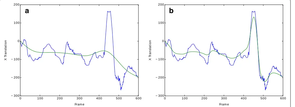
Figure4shows the trajectory generated by considering the horizontal translational factor (blue) and the obtained smoothing (green) using the Gaussian filter withσ = 40 and the adaptive version proposed in this work. It is pos-sible to observe that the smoothing is applied at different degrees along the trajectory.
3.5 Motion compensation and frame cropping
After applying the Gaussian filter, it is necessary to recalculate the value of each factor for each similarity matrix. In order to do that, the similarity matrix value of a given factor is calculated by the difference between each point of its smoothed trajectory and its predeces-sor. With the similarity matrices of each pair of frames updated, the similarity matrix is applied to the first frame of the pair to take it to the coordinates of the second.
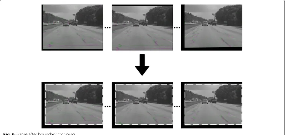
Applying the geometric transformation in the frame causes information to be lost in certain pixels of the frame boundary. Figure5presents a transformed frame, where it is possible to observe the loss of information at the bor-ders. They are then cropped so that no frames in the stabi-lized video hold pixels without information. To determine the frame boundaries, each similarity matrix is applied to the original coordinates of the four vertices, thus generat-ing the transformed coordinates for the respective frame. Finally, the innermost coordinates of all frames are con-sidered final. Figure6, extracted from [22], illustrates the cropping process applied to the transformed frame.
a
b
Fig. 5Frame after application of geometric transformation
3.6 Evaluation metrics
The peak signal-to-noise ratio (PSNR) is used to evalu-ate the overall difference between two frames of the video, expressed as
PSNR(ft,ft+1)=10 log10
WHL2 max W
x=1
H y=1
[ft(x,y)−ft+1(x,y)]2
(9)
where ft and ft+1 are two consecutive frames of the
video,W andHare the width and height of each frame, respectively, and Lmax is the maximum value intensity of the image. The PSNR metric is expressed in decibel (dB), a unit originally defined to measure sound intensity on a logarithmic scale. Typical PSNR values range from 20 to 40. The PSNR value should increase from the initial
video sequence to the stabilized sequence, since frames after transformation will tend to be more similar.
The interframe transformation fidelity (ITF) can be used to evaluate the final stabilization of the method, expressed as
ITF= 1 N−1
N−1
k=1
PSNR(k) (10)
whereNis the number of frames in the videos. Typically, the stabilized sequence has a higher ITF value than the original sequence.
Due to the loss of information in the application of the similarity matrix in the frames, it is important to evalu-ate and compare such revalu-ate among different stabilization methods. For this, we report the percentage of pixels held by the stabilized video in comparison to the original video, expressed as
Rate of preserved pixels=100WsHs
WH (11)
whereWandHcorrespond to the width and height of the frames in the original video andWsandHscorrespond to the width and height of the frames in the video generated by the stabilization process, respectively.
4 Results and discussion
This section describes the results of experiments con-ducted on a set of input videos. Fourteen videos with oscillations were submitted to the stabilization process and evaluated, where eleven of them are available from the
Table 1Video sequences used in our experiments
No. Video Source Resolution (pixels) FPS
1 gleicher1 GaTech VideoStab 640×360 30
2 gleicher2 GaTech VideoStab 640×360 30
3 gleicher3 GaTech VideoStab 640×360 30
4 gleicher4 GaTech VideoStab 640×360 30
5 greyson_chance GaTech VideoStab 640×360 30
6 hippo nghiaho.com/uploads/hippo.mp4 480×360 30
7 lf_juggle GaTech VideoStab 480×360 25
8 new_gleicher GaTech VideoStab 480×270 30
9 sam_1 GaTech VideoStab 640×360 30
10 sam and cocoa youtu.be/627MqC6E5Yo 540×360 30
11 sany0025 GaTech VideoStab 640×360 30
12 shake_pgh_1 GaTech VideoStab 640×360 30
13 shaky_car MatLab 320×240 30
14 yuna_long GaTech VideoStab 640×360 30
GaTech VideoStab [24] database and the three others col-lected separately. Table1presents the videos used in the experiments and their sources.
In the experiments performed, we compared the val-ues of the ITF metric as well as the amount of pixels held for different versions of the trajectory smoothing. In the first version, we used the Gaussian filter considering
σ =40. In another version, the Gaussian filter is used in a slightly more adaptive way, choosing different values ofσ
for each trajectory according to the size of the trajectory range with respect to the size of the video frame. Higher values ofσ are assigned to paths with smaller intervals; we then denominate this version as semi-adaptive. The locally adaptive version of the Gaussian filter proposed in this work is presented. A version using the Kalman filter is also shown. In addition, the videos were submitted to the YouTube stabilization method [24] in order to com-pare its results against ours. The metric is calculated for
Table 2Comparison between Gaussian filter and Kalman filter
No. of videos Original Gaussian filter Kalman filter
σ=40
ITF ITF Hold pixels (%) ITF Hold pixels (%)
1 18.793 27.738 69.276 25.888 71.000
2 20.390 29.331 71.750 27.201 74.771
3 16.186 22.559 72.972 22.122 73.003
4 19.965 33.380 48.958 26.298 54.903
5 23.277 28.660 2.540 25.991 4.958
6 19.681 29.804 67.891 25.576 73.507
7 24.109 28.510 60.495 28.063 57.167
8 17.881 25.448 70.648 24.081 72.287
9 19.248 23.251 25.797 21.426 33.818
10 12.972 18.453 17.519 16.680 27.204
11 21.487 26.826 43.599 25.704 52.875
12 15.081 0 0 20.219 2.686
13 23.841 30.621 70.312 28.200 71.875
14 18.065 20.265 7.448 20.902 7.642
Table 3Comparison between semi-adaptive Gaussian filter and adaptive Gaussian filter
No. of videos Original Semi-adaptive Gaussian filter Locally adaptive Gaussian filter
ITF ITF Hold pixels (%) ITF Hold pixels (%)
1 18.793 27.620 70.745 27.455 74.500
2 20.390 29.331 71.750 28.914 75.781
3 16.186 22.559 72.972 22.090 76.056
4 19.965 33.380 48.958 27.931 62.465
5 23.277 27.814 8.312 27.360 53.385
6 19.681 29.804 67.891 29.077 70.838
7 24.109 28.510 60.495 28.876 73.667
8 17.881 25.448 70.648 25.182 73.284
9 19.248 21.845 35.750 21.435 57.139
10 12.972 17.465 27.907 16.381 70.296
11 21.487 26.826 43.559 25.659 57.260
12 15.081 19.827 16.611 17.895 59.847
13 23.841 30.621 70.312 29.987 71.719
14 18.065 19.759 39.045 19.773 54.146
Average 19.355 25.772 50.353 24.858 66.455
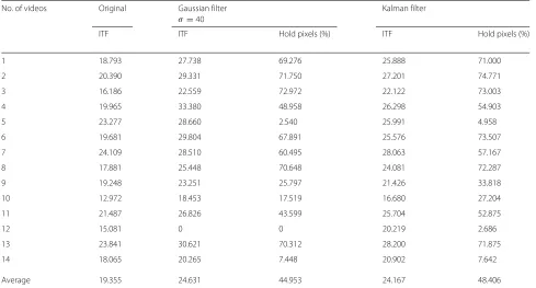
the video sequence before and after the stabilization pro-cess. Table2shows the results obtained with the Kalman filter and the Gaussian filter withσ=40.
From Table 2, we can observe a certain superiority in the use of the Gaussian filter, which achieves a higher ITF value for all videos with basically the same amount of pixels kept for most videos. Videos #5, #9, #10, #12, and #14 keep a lower amount of pixels compared to the other videos. This is due to the presence of desired
camera motion, which is erroneously considered as oscil-lations by the Gaussian filter, if the value of σ used is high enough. However, smaller values may not remove the oscillations from the videos efficiently, since each video has oscillations of different proportions.
In order to improve the quality of the stabilization for these cases, Table 3 presents the results obtained with the version of the semi-adaptive Gaussian filter, where trajectories with greater difference between the
Table 4Comparison between adaptive Gaussian filter and YouTube method [24]
No. of videos Original Locally adaptive Gaussian filter YouTube [24] Hold pixels
1 18.793 27.455 27.890 Superior
2 20.390 28.914 28.604 Superior
3 16.186 22.090 23.030 Comparable
4 19.965 27.931 33.711 Superior
5 23.277 27.360 27.599 Inferior
6 19.681 29.077 29.390 Superior
7 24.109 28.876 29.252 Comparable
8 17.881 25.182 25.908 Superior
9 19.248 21.435 20.922 Inferior
10 12.972 16.381 20.495 Superior
11 21.487 25.659 26.672 Comparable
12 15.081 17.895 19.283 Comparable
13 23.841 29.987 28.845 Comparable
14 18.065 19.773 20.128 Inferior
Fig. 7Video#1. Amount of pixels hold through our method is superior than the state-of-the-art approach.aAdaptive Gaussian filter;bYouTube [24]
minimum and maximum values will have a lower value for σ. We used σ = 40 for trajectories with inter-vals smaller than 80% of the respective frame size, whereas σ = 20 otherwise. For the locally adap-tive version proposed in this work, we experimen-tally set rmin as 0.4, whose results are reported in
Table3.
The semi-adaptive version maintains more pixels in the videos in which the original Gaussian filter had prob-lems, sinceσ = 20 was applied to them. However, the amount of pixels held in the frames is lower than in the other videos. This is because, in many cases,σ = 20 is still a very high value. On the other hand, smaller values ofσ can ignore the oscillations that are present in other instance of the video, thus generating videos not stabi-lized enough and consequently with a lower ITF value. Therefore, as can be seen in Table 3, the locally adap-tive version, whose smoothing intensity is changed along the trajectory, obtained ITF values comparable to the original and semi-adaptive version, maintaining consider-ably more pixels.
Table 4presents a comparison of the results between our method and YouTube approach [24]. The percentage of pixels held was not reported since the YouTube method resizes the stabilized videos to their original size. Thus, a qualitative analysis is done through the first frame of each video, whose results are classified into three categories: superior (when our method maintains more pixels), infe-rior (when the YouTube method holds more pixels), and
comparable (when both methods hold basically the same amount of pixels). Figures7,8, and9illustrate the analysis performed.
In Fig. 7, it is possible to observe that more infor-mation is maintained on the top, left, and right sides of the video obtained with our method. The difference is not considerably large, and the advantage or dis-advantage obtained follows these proportions in most videos.
In Fig.8, there is less information maintained on the top and bottom sides in the use of the adaptive Gaussian filter. On the other hand, there is a larger amount of information held on the left and right sides.
Figure9illustrates a situation where our method main-tains less pixels. Lower amount of information is held on the every sides with our method.
From Table 4, we can observe a certain parity for both methods in terms of ITF metric, with a slight advantage of the YouTube method [24], while the main-tained pixels are in general comparable and, when lower, do not differ much. This demonstrates that the pro-posed method is competitive with one of the meth-ods considered as current state-of-the-art, despite the simplicity of our method. Notwithstanding, the method still needs to be further extended to deal with some adverse situations, such as the treatment of non-rigid oscillations in the video #10, the rolling shut-ter in the video #12, and the parallax effect, among others.
Fig. 9Video#12. Amount of pixels hold through our method is inferior than the state-of-the-art approach.aAdaptive Gaussian filter;bYouTube [24]
5 Conclusions
In this work, we presented a technique for video stabi-lization based on an adaptive Gaussian filter to smooth the camera trajectory in order to remove undesired oscil-lations. The proposed filter assigns distinct values to σ along the camera trajectory by considering that the inten-sity of the oscillations changes throughout the video and that a very high value ofσ can result in a video with a low amount of pixels, while smaller values generate less stabilized videos.
The results obtained in the experiments were compared with different versions for the smoothing of the trajec-tory: Kalman filter, Gaussian filter withσ = 40, and a semi-adaptive Gaussian filter. The approaches achieved comparable values for the ITF metric while maintaining a significantly higher amount of pixels.
A comparison was performed with the stabilization method used in YouTube, where the results were compet-itive. As directions for future work, we intend to extend our method to deal with some adverse situations, such as non-rigid oscillations and effect of parallax.
Abbreviations
2D: Two-dimensional; 3D: Three-dimensional; CMOS: Complementary metal oxide semiconductor; CV: Coefficient of variation; dB: Decibel; ITF: Interframe transformation fidelity; MSE: Mean square error; PSNR: Peak signal-to-noise ratio; RANSAC: Random sample consensus; SFM: Structure-from-motion
Acknowledgements
The authors would like to thank the editors and anonymous reviewers for their valuable comments.
Funding
The authors are thankful to FAPESP (grants #2014/12236-1 and
#2017/12646-3) and CNPq (grant #305169/2015-7) for their financial support.
Availability of data and materials
Data are publicly available.
Authors’ contributions
HP and MRS contributed equally to this work. Both authors carried out the in-depth analysis of the experimental results and checked the correctness of the evaluation. Both authors took part in the writing and proof reading of the final version of the paper. Both authors read and approved the final manuscript.
Competing interests
The authors declare that they have no competing interests.
Publisher’s Note
Springer Nature remains neutral with regard to jurisdictional claims in published maps and institutional affiliations.
Received: 28 November 2017 Accepted: 15 May 2018
References
1. C Yan, Y Zhang, J Xu, F Dai, J Zhang, Q Dai, et al., Efficient parallel framework for HEVC motion estimation on many-core processors. IEEE Trans. Circ. Syst. Video Technol.24(12), 2077–2089 (2014)
2. MF Alcantara, TP Moreira, H Pedrini, Real-time action recognition using a multilayer descriptor with variable size. J. Electron. Imaging.25(1), 013020.1?013020.9 (2016)
3. C Yan, Y Zhang, J Xu, F Dai, L Li, Q Dai, et al., A highly parallel framework for HEVC coding unit partitioning tree decision on many-core processors. IEEE Sig. Process. Lett.21(5), 573–576 (2014)
4. MF Alcantara, H Pedrini, Y Cao, Human action classification based on silhouette indexed interest points for multiple domains. Int. J. Image Graph.17(3), 1750018_1–1750018_27 (1750)
5. C Yan, H Xie, D Yang, J Yin, Y Zhang, Q Dai, Supervised hash coding with deep neural network for environment perception of intelligent vehicles. IEEE Trans. Intell. Transp. Syst.19(1), 284–295 (2018)
6. MF Alcantara, TP Moreira, H Pedrini, F Fl´rez-Revuelta, Action identification using a descriptor with autonomous fragments in a multilevel prediction scheme. Signal Image Video Process.11(2), 325–332 (2017)
7. C Yan, H Xie, S Liu, J Yin, Y Zhang, Q Dai, Effective Uyghur language text detection in complex background images for traffic prompt
identification. IEEE Trans. Intell. Transp. Syst.19(1), 220–229 (2018) 8. BS Torres, H Pedrini, Detection of complex video events through visual
rhythm. Vis. Comput.34(2), 145–165 (2018)
9. MVM Cirne, H Pedrini, inProgress in Pattern Recognition, Image Analysis, Computer Vision, and Applications. A video summarization method based on spectral clustering (Springer, 2013), pp. 479–486
10. MVM Cirne, H Pedrini, inProgress in Pattern Recognition, Image Analysis, Computer Vision, and Applications. Summarization of videos by image quality assessment (Springer, 2014), pp. 901–908
11. TS Huang,Image Sequence Analysis. vol. 5. (Springer Science & Business Media, Heidelberg, 2013)
12. AA Amanatiadis, I Andreadis, Digital image stabilization by independent component analysis. IEEE Trans. Instrum. Meas.59(7), 1755–1763 (2010) 13. JY Chang, WF Hu, MH Cheng, BS Chang, Digital image translational and rotational motion stabilization using optical flow technique. IEEE Trans. Consum. Electron.48(1), 108–115 (2002)
14. S Ertürk, Real-time digital image stabilization using Kalman filters. Real-time Imaging.8(4), 317–328 (2002)
15. R Jia, H Zhang, L Wang, J Li, inInternational Conference on Artificial Intelligence and Computational Intelligence. Digital image stabilization based on phase correlation. vol. 3 (IEEE, 2009), pp. 485–489 16. SJ Ko, SH Lee, KH Lee, Digital image stabilizing algorithms based on
bit-plane matching. IEEE Trans. Consum. Electron.44(3), 617–622 (1998) 17. S Kumar, H Azartash, M Biswas, T Nguyen, Real-time affine global motion estimation using phase correlation and its application for digital image stabilization. IEEE Trans. Image Process.20(12), 3406–3418 (2011) 18. CT Lin, CT Hong, CT Yang, Real-time digital image stabilization system
using modified proportional integrated controller. IEEE Trans. Circ. Syst. Video Technol.19(3), 427–431 (2009)
20. C Morimoto, R Chellappa, in13th International Conference on Pattern Recognition. Fast electronic digital image stabilization. vol. 3 (IEEE, 1996), pp. 284–288
21. YG Ryu, MJ Chung, Robust online digital image stabilization based on point-feature trajectory without accumulative global motion estimation. IEEE Signal Proc. Lett.19(4), 223–226 (2012)
22. Y Matsushita, E Ofek, W Ge, X Tang, HY Shum, Full-frame video stabilization with motion inpainting. IEEE Trans. Pattern Anal. Mach. Intell.
28(7), 1150–1163 (2006)
23. S Liu, L Yuan, P Tan, J Sun, Bundled camera paths for video stabilization. ACM Trans. Graph.32(4), 78 (2013)
24. M Grundmann, V Kwatra, I Essa, inIEEE Conference on Computer Vision and Pattern Recognition. Auto-directed video stabilization with robust L1 optimal camera paths (IEEE, 2011), pp. 225–232
25. C Jia, BL Evans, Online motion smoothing for video stabilization via constrained multiple-model estimation. EURASIP J. Image Video Proc.
2017(1), 25 (2017)
26. S Liu, M Li, S Zhu, B Zeng, CodingFlow: enable video coding for video stabilization. IEEE Trans. Image Proc.26(7), 3291–3302 (2017) 27. Z Zhao, X Ma, inIEEE International Conference on Image Processing. Video
stabilization based on local trajectories and robust mesh transformation (IEEE, 2016), pp. 4092–4096
28. N Bhowmik, V Gouet-Brunet, L Wei, G Bloch, inInternational Conference on Multimedia Modeling. Adaptive and optimal combination of local features for image retrieval (Springer, Cham, 2017), pp. 76–88
29. H Guo, S Liu, S Zhu, B Zeng, inIEEE International Conference on Image Processing. Joint bundled camera paths for stereoscopic video stabilization (IEEE, 2016), pp. 1071–1075
30. Q Zheng, M Yang, A video stabilization method based on inter-frame image matching score. Glob. J. Comput. Sci. Technol.17(1), 41–46 (2017) 31. S Liu, B Xu, C Deng, S Zhu, B Zeng, M Gabbouj, A hybrid approach for
near-range video stabilization. IEEE Trans. Circ. Syst. Video Technol.27(9), 1922–1933 (2016)
32. BH Chen, A Kopylov, SC Huang, O Seredin, R Karpov, SY Kuo, et al., Improved global motion estimation via motion vector clustering for video stabilization. Eng. Appl. Artif. Intell.54, 39–48 (2016)
33. B Cardani, Optical Image Stabilization for Digital Cameras. IEEE Control. Syst.26(2), 21–22 (2006)
34. C Buehler, M Bosse, L McMillan, inIEEE Computer Society Conference on Computer Vision and Pattern Recognition. Non-metric image-based rendering for video stabilization. vol. 2 (IEEE, 2001), pp. II–609
35. G Zhang, W Hua, X Qin, Y Shao, H Bao, Video Stabilization based on a 3D Perspective Camera Model. Vis. Comput.25(11), 997–1008 (2009) 36. KY Lee, YY Chuang, BY Chen, M Ouhyoung, inIEEE 12th International
Conference on Computer Vision. Video stabilization using robust feature trajectories (IEEE, 2009), pp. 1397–1404
37. HC Chang, SH Lai, KR Lu, inIEEE International Conference on Multimedia and Expo. A robust and efficient video stabilization algorithm. vol. 1 (IEEE, 2004), pp. 29–32
38. G Puglisi, S Battiato, A robust image alignment algorithm for video stabilization purposes. IEEE Trans. Circ. Syst. Video Technol.21(10), 1390–1400 (2011)
39. S Battiato, G Gallo, G Puglisi, S Scellato, in14th International Conference on Image Analysis and Processing. SIFT features tracking for video stabilization (IEEE, 2007), pp. 825–830
40. Y Shen, P Guturu, T Damarla, BP Buckles, KR Namuduri, Video stabilization using principal component analysis and scale invariant feature transform in particle filter framework. IEEE Trans. Consum. Electron.55(3), 1714–1721 (2009)
41. BY Chen, KY Lee, WT Huang, JS Lin, Wiley Online Library. Capturing intention-based full-frame video stabilization. Comput. Graphics Forum.
27(7), 1805–1814 (2008)
42. S Ertürk, Image sequence stabilisation based on Kalman filtering of frame positions. Electron. Lett.37(20), 1 (2001)
43. A Litvin, J Konrad, WC Karl, inElectronic Imaging.International Society for Optics and Photonics. Probabilistic video stabilization using Kalman filtering and mosaicing (SPIE-IS&T, 2003), pp. 663–674
44. J Yang, D Schonfeld, C Chen, M Mohamed, inInternational Conference on Image Processing. Online video stabilization based on particle filters (IEEE, 2006), pp. 1545–1548
45. ML Gleicher, F Liu, Re-cinematography: improving the camerawork of casual video. ACM Trans. Multimed. Comput. Commun. Appl.5(1), 2 (2008) 46. J Bai, A Agarwala, M Agrawala, R Ramamoorthi, Wiley Online
Library.User-assisted video stabilization. Comput. Graph. Forum.33(4), 61–70 (2014)
47. F Liu, M Gleicher, J Wang, H Jin, A Agarwala, Subspace video stabilization. ACM Trans. Graph.30(1), 4 (2011)
48. P Bhat, CL Zitnick, N Snavely, A Agarwala, M Agrawala, M Cohen,et al, in 18th Eurographics Conference on Rendering Techniques. Eurographics Association. Using photographs to enhance videos of a static scene, (2007), pp. 327–338
49. F Liu, M Gleicher, H Jin, A Agarwala, Content-preserving warps for 3D video stabilization. ACM Trans. Graph.28(3), 44 (2009)
50. F Liu, Y Niu, H Jin, inIEEE International Conference on Computer Vision. Joint subspace stabilization for stereoscopic video, (2013), pp. 73–80 51. A Goldstein, R Fattal, Video stabilization using epipolar geometry. ACM
Trans. Graph.31(5), 1–10 (2012)