A hierarchical graph model for object cosegmentation

R E S E A R C H

Open Access

A hierarchical graph model for object

cosegmentation

Yanli Li, Zhong Zhou

and Wei Wu

Abstract

Given a set of images containing similar objects, cosegmentation is a task of jointly segmenting the objects from the set of images, which has received increasing interests recently. To solve this problem, we present a novel method based on a hierarchical graph. The vertices of the hierarchical graph involve pixels, superpixels and heat sources, and cosegmentation is performed as iterative object refinement in the three levels. With the inter-image connection in the heat source level and the intra-image connection in the superpixel level, we progressively update the object

likelihoods by transferring message across images via belief propagation, diffusing heat energy within individual image via random walks, and refining the foreground objects in the pixel level via guided filtering. Besides, a histogram based saliency detection scheme is employed for initialization. We demonstrate experimental evaluations with state-of-the-art methods over several public datasets. The results verify that our method achieves better segmentation quality as well as higher efficiency.

Keywords: Cosegmentation, Hierarchical graph, Heat source, Saliency detection, Belief propagation, Random walks, Guided filtering

1 Introduction

The term “cosegmentation” is first introduced by Rother et al. [1] in 2006, referring to the problem of simultane-ously segmenting “similar” foreground objects in a set of images. The definition of “similar” commonly indicates the constraint that the distribution of some appearance cues such as color and texture in each image has to be sim-ilar. Cosegmentation has many potential applications. It can be used for summarizing personal photo album, guid-ing multiple images’ editguid-ing, boostguid-ing unsupervised object recognition, improving content based image retrieval and so on.

Since the introduction of the problem, various methods have been presented. One type of methods handles the problem of multi-class cosegmentation, while others focus on binary cosegmentation. In this article, we are interested in binary cosegmentation and observe that for most appli-cations of binary cosegmentation several criteria should be followed: (1) automation, i.e., it is executed without user interactions; (2) scalability, i.e., it can be applied to

*Correspondence: [email protected]

State Key Laboratory of Virtual Reality Technology & Systems, Beihang University, Beijing, China

hundreds of images instead of two images or small sized image sets; (3) focusing on “object” instead of “stuff ”. Here the “object” refers to “foreground things” such as a person or a bird, while “stuff ” refers to “background regions” such as road or sky; (4) high segmentation accuracy; (5) low running time. According to these criteria, existing meth-ods have some limitations. For example, the iCoseg system presented by Batra et al. [2] can obtain highly accurate results, but requires user input. The methods reviewed by Vicente et al. [3] all focus on cosegmenting two images. The recently presented CoSand [4] only extracts similar large regions, thus it often omits the small foreground objects in the images. Methods based on topic discovery like [5-7] all take superpixels as computation nodes, and hence they suffer from detail loss because superpixels tend to merge foreground regions with the backgrounds. Some unsupervised object segmentation methods [8-11] extract objects from multiple images via iteratively learning class models and segmenting objects in pixel level, while they are time-consuming because the employed optimization schemes like graphcut [12] and belief propagation [13] are inefficient with a large number of pixel nodes.

In this article, we try to meet these criteria by extract-ing the foreground objects with a three-level hierarchical

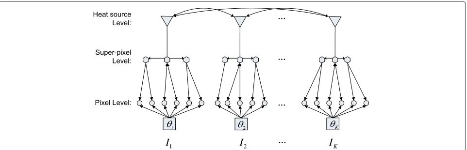
graph model. As shown in Figure 1, the graph model is composed of the pixel, superpixel and heat source lev-els, in which superpixels are grouping units of pixels obtained by an over-segmentation method [14] and heat sources are the representative superpixels obtained by a bottom-up agglomerative clustering scheme. The term “heat source” is introduced in random walks [15], repre-senting heat energy convergence points. Here, we adopt it to describe message transferring among images and heat energy diffusion within individual image. The itera-tive object refinement is operated at the three levels with different optimization schemes. The heat source level uti-lizes belief propagation [13] for message transferring. In the superpixel level, random walks [15] is employed for heat energy diffusion. In the pixel level, we refine the foreground objects within each image via guided filter-ing [16]. By dofilter-ing so, the foreground objects are grad-ually extracted. Besides, we employ a histogram based saliency detection method [17] for initializing the object likelihoods.

It is no doubt that our method is automatic and has the following advantages. (1) It is scalable. Since the super-pixel and super-pixel levels both treat each image separately, and the heat source level’s integration only operates on limited heat sources, this method has high parallelization capacity and can be easily applied to large scale image collection. (2) It focuses on “object” instead of “stuff ”. This is because our method is initialized by saliency detection, which can filter out background stuff. (3) It is computationally more efficient. Compared with meth-ods [8,9,18] which perform message transferring among images using a large number of superpixels or pixels, our method uses a small number of heat sources and thus sig-nificantly reduce computation time. (4) It can preserve object boundaries. This method finally refines object segmentation in the pixel level, and hence avoids the

problem of detail loss existing in other superpixel based methods.

The remainder of this article is organized as follows. After summarizing the related study in Section 2, we present the hierarchical graph model in Section 3. The stages of object refinement along the model, including foreground initialization, local object refinement, mes-sage transferring and heat energy diffusion are described in Section 4. Experimental results are demonstrated in Section 5, and we conclude the article in the last section.

2 Related work

Basically, the solutions to cosegmentation can be roughly classified into two categories: clustering based methods [5-7,19] and labeling based methods [3,8-11,18]. The for-mer tries to partition nodes (pixels or superpixels) in the images into distinct, semantically coherent clusters, while the latter aims at assigning each node with a unique label.

2.1 Clustering based methods

Under the assumption that similar objects often recur in multiple images, clustering based methods employ clus-tering models to discover such frequent regions. The well-known clustering models include topic discovery models like probabilistic latent semantic analysis (PLSA) [20], and geometry based models like normalized cuts (NCut) [21]. Motivated by the success of topic discovery in text analysis, Russell et al. [5] first adopt PLSA to address the cosegmentation problem. Later, Cao et al. [6] and Zhao et al. [7] both present spatially coherent topic models to encode the spatial relationship of image patches which is ignored by the traditional topic models. Combining NCut and supervised classification technique, Joulin et al. [19] utilize a discriminative clustering scheme to tackle the cosegmentation problem. For speeding up, all clustering based methods take superpixels as computation

1 2 K

K

I

2

I

1

I

nodes. The major limitation of these methods is the lower segmentation accuracy caused by the over-segmentation methods.

2.2 Labeling based methods

Considering the Markov property in the images, labeling based methods formulate cosegmentation as a Markov random field (MRF) energy minimization problem. Over the past decade, methods that use graphcut [12] to min-imize MRF energy have become the standard for figure-ground separation.

One technique is to minimize an energy function that is a combination of a pairwise MRF energy and a his-togram matching term. The hishis-togram matching terms such as L1 norm model [1], L2 norm model [22] and “reward” model [23] force foreground histograms between a pair of images to be similar. Vicente et al. [3] review these models and make a comparison. Yet these meth-ods are limited to two images. Another technique, also called unsupervised object segmentation such as LOCUS [8], ClassCut [9], Arora et al. [10] and Chen et al. [11], per-forms object cosegmentation by iteratively learning the object geometric models and segmenting the foreground objects. The initialization stages of these methods play an important role for energy minimization. For example, LOCUS [8] takes the pre-trained mask and edge proba-bility maps as the initial object models, ClassCut [9] uses a general object detector [24] to locate objects. However, these methods are limited to segmenting objects with sim-ilar geometric shape. In contrast, the recently proposed cosegmentation method—BiCos [18] is more general and can be applicable for any non-rigid objects. BiCos [18] operates at the two levels: the bottom level treats each image separately and uses graphcut [12] to refine fore-ground objects in pixel level, whereas the top level takes superpixels as computation units and employs a dis-criminative classification to propagate information among images.

Our method falls into the last category. The main idea is to combine multiple schemes along a three-level hier-archical graph to refine foreground objects successively. In contrast to other labeling based methods [3,8-11,18], this method has the following characteristics: (1) uti-lization of heat sources for message propagation among images, which can significantly reduce computation time; (2) a saliency detection based initialization, which can remove the impact of background stuff; (3) instead of using graphcut [12] to refine objects in the pixel level, we introduce guided filtering [16] for local refinement. In experiments, we compare our method quantitatively and qualitatively with other state-of-the-art methods over sev-eral public datasets. As a outcome, our method achieves better segmentation quality as well as lower computation time.

3 The hierarchical graph model

3.1 Problem formulation

Given a set of images containing objects of the same class,I = {I_k,k = 1,. . .,K}, the goal of cosegmentation is to simultaneously extract the foreground objects. We formulate this problem as a binary labeling: L = {Lk, k = 1,. . .,K}, which assigns each pixelxin the imageIk

with a labelLk(x). Lk(x) = 0 indicatesx belongs to the

background, whereasLk(x) = 1 to the foreground. The

best labeling follows maximum a posteriori estimation, i.e.,L∗ = arg max_Lp(L|I). Based on the Bayesian per-spective,p(L|I)∝p(L)p(I|L), wherep(L)is the labeling prior andp(I|L)is the observation likelihood. Under the assumption that the prior follows uniform distribution and the observation likelihood is pair-wise dependent among images, the posteriori can be rewritten as:

p(L|I)∝ k

p(Ik|Lk)

(k1,k2)

p(Ik1,Ik2|Lk1,Lk2) (1)

The corresponding energy function (i.e., E(x) = −

logp(x)) is:

E(L|I)= k

Ed(Ik|Lk)+

(k1,k2)

Es(Ik1,Ik2|Lk1,Lk2) (2)

The energy function combines the unary terms Ed(·)

and the pairwise terms Es(·,·). In our study, the unary

term is composed of two parts:

Ed(Ik|Lk)=Ed1(Ik|Lk)+Ed2(Ik|Lk,θk) (3)

whereEd1(Ik|Lk)is derived from saliency detection, and Ed2(Ik|Lk,θk) is inferred under the guide of an inherent

object model.θ_kis the latent parameter set for the object model ofIk.

The pairwise term can be considered as a smooth term, which penalizes the inconsistent labeling among images. Ideally, this term should be formulated in the pixel level. For computational efficiency, we define it in the heat source level using appearance information (see Equation (8)). Minimizing the above energy with respect to all discrete labels is intractable. Instead, we relax the labels firstly, i.e., letLk(x)∈[ 0, 1] be the object

likelihood, and iteratively update them along a hierarchi-cal graph model, finally obtain the segmentation results by rounding.

3.2 The hierarchical graph and our method

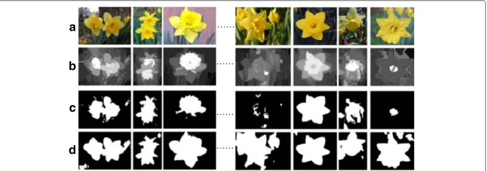
Figure 2Saliency detection based model initialization.(a)The input image,(b)the saliency detection result,(c)the segmentation result built on GMM, and(d)the segmentation result obtained after guided filtering.

implementation, the superpixels are extracted by an over-segmentation method—Turbopixels [14]. The generation of heat sources will be described in detail in Section 4.2.

Based on the graph model, our method successively updates the object likelihoods by the following iteration: (1) estimating the latent parameters and refining object segmentation, (2) transferring message among images and diffusing heat energy within individual image. Specif-ically, we first obtain the object likelihoods in each image with saliency detection [17], and then estimate the latent parameters to update the object likelihoods. The like-lihoods of the heat sources are further updated among images via message transferring which is fulfilled by belief propagation [13], and diffused to other superpixels using random walks [15] within individual image. Now the likelihoods can be considered as input for further iter-ation. In the following sections, we denote the updated object likelihoods at different stages byL∗_k,t,t = 0,. . ., 3, k = 1,. . .,K. To summarize the cosegmenta-tion method presented in this article, we provide a high level overview of the method pipeline as follows.

• Input:a set of images containing objects of the same classI= {I_k,k=1,. . .,K}

• Output:the cosegmentation results with the form of binary labelingL∗= {L∗_k,k=1,. . .,K}

Step 1. Initialization (Section 4.1)

a)partition each imageIkinto a set of superpixelsSk

and extract heat sourcesZk.

b)obtain the initial object likelihoodsL∗_k,0via saliency detection [17].

c)estimate the latent parameter setθ_k.

d)acquire the updated object likelihoodsL∗_k,1via guided filtering [16].

Step 2. Global message transferring (Section 4.2)

Optimize the energy function defined in

Equation (6) via belief propagation [13] to provide the updated object likelihoodsL∗,2(Z)for all heat sources.

Step 3. Local heat energy diffusion (Section 4.3)

For each imageIk, the object likelihoods of the heat

sourcesL∗_k,2(Zk)are diffused to other superpixels

Uk=Sk−Zkvia random walks [15], obtaining L∗_k,2(U_k).

Step 4. Local object refinement (Section 4.1)

a)letL∗_k,3=(L∗_k,0+L∗_k,1+L∗_k,2)/3.

b)re-estimate the latent parameter setθ_k.

c)acquire the updated object likelihoodsL∗_k,1via guided filtering [16].

Step 5.Repeat Step 2, 3, and 4 until convergence. The final labelingL∗_kis obtained by binarizingL∗_k,3.

4 Hierarchical graph based object cosegmentation

4.1 Initialization and local refinement

One major visual characteristic of objects is that they often stand out as saliency [24]. Based on this character-istic, we apply saliency detection to initially detect fore-ground regions in each image. Over various of saliency detection methods, we choose a recently proposed his-togram based method [17] for its efficiency and effective-ness. Figure 2b demonstrates the saliency detection result of Figure 2a. We define the initial object likelihoodsL∗_k,0as the saliency likelihoods.

The segmentation results obtained by thresholding saliency likelihoods often contain holes and ambiguous boundaries. Motivated by the interactive segmentation methods, e.g., GrabCut [25], we utilize the inherent color Gaussian mixture model (GMM) in the image to update the object likelihoods. Two GMMs, one for the foreground and another for the background, are esti-mated in RGB color space. Each GMM is taken to be a full-covariance Gaussian mixture with M com-ponents. The GMM parameters are defined as: θ_k = {θ_kJ|J ∈ {B,F}}, in which θ_kJ = {θ_mJ_,k|m = 1,. . .,M},

θ_mJ_,k = (μJ_m,k,_mJ_,k,ωJ_m,k). (μF_m,k,_mF_,k,ωF_m,k) are the mean, covariance and weighting values for the foreground components, and (μB_m,k,_mB_,k,ωB_m,k) for the background components. The GMM parameters are estimated from the initial likelihoods as follows: (1) given two thresholds T1andT2, satisfying 0 <T1< T2< 1, we label the

pix-els withL∗_k,0(x) >T1as foreground, whereasL∗_k,0(x) <T2

……

……

……

……

a

b

c

d

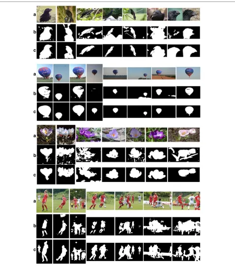
Figure 3The segmentation results obtained before and after message transferring.(a)The input images,(b)the saliency detection results, (c)the segmentation results obtained in the initial stage, and(d)the segmentation results obtained after message transferring.

statistically acquire its parametersθ_mJ_,k. The object likeli-hoods built on the GMMs are given by:

p(Ik(x)|θ_kJ)=max

m (p(Ik(x)|θ J

m,k)) (4)

p(Ik(x)|θ_mJ_,k)=ωJ_m,kexp(−Ik(x)−μ_mJ _,k/_mJ _,k)/

|_mJ _,k|

(5)

Segmenting objects by directly thresholding the updated object likelihoods will result in noises, as shown in Figure 2c. We use guided filtering [16] to remove noises. The main idea of guided filtering [16] is that, given the filter inputp, the filter outputqis locally linear to the guidance mapI, qi = axIi +bx,∀i ∈ wx, wherewx is a

window with radiusrcentered at the pixelx. By minimiz-ing the difference between the filter inputpand the filter outputq, i.e.,Err(ax,bx) = i∈wx((pi−qi)2+a2x), we

can obtainax,bxand the filter outputq.

Based on guided filtering [16], we perform local refine-ment with three steps: (1) obtaining the foreground likelihood mapLk,F = {p(Ik(x)|θ_kF)}and the background

likelihood map Lk,B = {p(Ik(x)|θkB)}; (2) taking the

grayscale image ofI_k as the guidance map, the two like-lihood maps are filtered, respectively (denoting the filter outputs asLˆk,F andLˆk,B); (3) defining the refined object

likelihoods asL∗_k,1 = ˆLk,F/(Lˆk,F+ ˆLk,B). Figure 2d shows

the refinement result of Figure 2c. As can be seen, the guided filtering based scheme can significantly improve segmentation quality.

4.2 Global message transferring

Due to the diversity of realistic scenes, saliency based object segmentation sometimes fails to extract objects of the same class (see Figure 3c). The seg-mentation quality can be further boosted by sharing appearance similarity among images. Unlike other cosegmentation methods [8,9,18] which propagate the distributions of visual appearance in the pixel or superpixel level, we perform message propaga-tion in the heat source level to reduce computapropaga-tion time.

As stated in Section 3, heat sources are the represen-tative superpixels located in the centers of the cluster-ing regions formed by coherent superpixels. The regions are formed by a bottom-up agglomerative clustering scheme. Specifically, given an imageI, we first partition it into a collection of superpixels via Turbopixels [14] (see Figure 4b, in which superpixels are encircled with red boundaries). Then we build an intra-image graph GS = < S,YS >, where S = {si} is the superpixel set and YS = {(si,sj)} is the edge set connecting all pairs of

adjacent superpixels. The edge weight is defined by Gaus-sian similarity between the normalized mean RGB color of the nodes, i.e., w(si,sj) = exp(−I(si) − I(sj)2)/σs,

whereσs is a variance constant. Based on the graphGS,

we use a greedy scheme to merge nodes one by one. Each time, we select the edge with the maximum weight value and merge its two nodes. This step is repeated until all nodes are merged into N regions. The central superpixel of each region is chosen as a heat source. Figure 4c demonstrates the clustering regions overlaid by the heat sources, in which the regions are encircled with green boundaries and the heat sources are colored in blue.

For message transferring among images, we construct an inter-image graphGZ = < Z,YZ >.GZ is an

undi-rected complete graph, where Z = {zi|zi ∈ Zk,k =

1,. . .,K}includes all heat sources from the input images, YZ = {(zi,zj)} connects all pairs of heat sources. We

update the object likelihoods of the heat sources by mini-mizing a standard MRF energy function that is the sum of unary termsE1(·)and pairwise termsE2(·,·):

E(L(Z))= zi∈Z

E1(zi)+λ

(zi,zj)∈YZ

E2(zi,zj) (6)

where λ is the weighting value balancing the trade off between the unary terms and the pairwise terms.

The unary termE1(·) imposes individual penalties for

assigning any likelihood L(zi) to the heat sourcezi. We

rely on the object likelihoodsL∗,1acquired in the previous stage to define this term:

E1(zi)= L(zi)−

x∈zi

L∗,1(x)/|zi|

(7)

The pairwise termE2(·,·)defines to what extent

adja-cent heat sources should agree. It often depends on local observation. In our study, the pairwise potential takes the form:

E2(zi,zj)=w(zi,zj)|L(zi)−L(zj)| (8)

where w(zi,zj)is the edge weight, defined asw(zi,zj) =

exp(−f(zi)−f(zj)2)/σz,σzis a variance constant.f(z)

is a nine-dimensional descriptor for the heat source z, including three-dimensional mean Lab color feature, four-dimensional mean texture featurea and two-dimensional mean position feature. This definition suggests that the larger the weight for the edge, the more similar the labels for its two nodes.

We utilize belief propagation [13] to optimize the energy function in several bounds. The main idea of belief prop-agation is to iteratively update a set of message maps between neighboring nodes. The message maps that are denoted by {mt_zi→zj(L(zj)),t = 1,. . .,T} represent the

transferred message from one node to another at each

iteration. In our study, the message maps are initially set to zero and updated as follows:

mt_zi→zj(L(zj))=min L(zi)

⎛

⎝E1(zi)+λE2(zi,zj)+

zk∈Z/zj

mt−_zk→z1 _i(L(zi)) ⎞ ⎠

(9)

Finally, a belief vector is computed for each node, bzi(L(zi)) = E1(zi) +

zj∈Zm

T

zj→zi(L(zi)), and the

updated object likelihoods are expressed as: L∗,2(zi) = bzi(0)/(bzi(0)+bzi(1)).

4.3 Local heat energy diffusion

After global message transferring, the object likelihoods for heat sources preserve appearance similarity among images. We further diffuse them to other superpixels. As illustrated in the middle level of Figure 1, this is performed by heat energy diffusion within individual image. The heat energy diffusion can be imagined in the following situa-tion: putting some heat sources in a metal plate, the heat energy will diffuse to other points as time goes by, finally each point will have a stable temperature. How to calcu-late such steady-state temperatures? This is a well-known Dirichlet energy minimization problem:

u∗=arg min

u (E(u))=arg minu

1 2

u∈

|∇u|2d (10)

Grady [15] states the similar problem in discrete space with the term “random walks”. Based on a graph GX = < X,YX >, where X = {xi}

is the node set and YX = {(xi,xj)} is the set of

node pairs, the Dirichlet energy function takes the form:

E(u(X))= 1

2

(xi,xj)∈YX

w(xi,xj)(u(xi)−u(xj))2 (11)

where w(xi,xj) is the edge weight for the adjacent node

pair(xi,xj).

In our study, the random walks works on the graph GS_k =< Sk,Y_kS >for the imageIk, whereSk = {si}is the

superpixel set andY_kS = {(si,sj)}is the edge set

connect-ing all pairs of adjacent superpixels. The correspondconnect-ing energy function is:

E(L(Sk))=

1 2

(si,sj)∈YkS

w(si,sj)(L(si)−L(sj))2

= 1

2L(Sk)

T_QL(S k)

(12)

whereQ= D−Ais the Laplacian matrix, in whichA = {w(si,sj)} is the edge weight matrix, andDis a diagonal

We divide the node set Sk into two parts: the heat

sourcesZkand the superpixelsUk =Sk−Zk. The energy

function can be rewritten as:

E(L(Sk))=

L(Zk)T,L(Uk)T

QZk B

BT QUk

L(Zk) L(Uk)

(13)

whereQZk andQUk correspond to the Laplacian matrix

for the node setZkandUk, respectively.

Minimizing E(L(Sk)) is equal to

differentiat-ing E(L(Sk)) with respect to L(Uk) and yields: L(U_k)= −BT_L(Z

k)/QUk.L(Zk)are the object likelihoods

acquired in the previous stage, i.e., L(Zk) = L∗,2(Zk).

The diffused object likelihoods for Uk are obtained by: L∗,2(Uk) = −BTL∗,2(Zk)/QUk. The nonsingularity ofQUk

guarantees that the solution exists and is unique.

For each pixelx, its object likelihoodL∗,2(x)is assigned as the object likelihood of the superpixel it belongs to. TakingL∗_k,3(x)=(L∗_k,0(x)+L∗_k,1(x)+L∗_k,2(x))/3 as input, we further invoke local refinement (see Section 4.1) to opti-mize object segmentation. Figure 3 demonstrates the seg-mentation results obtained before and after heat energy diffusion. As can be seen, although the saliency based initialization stage sometimes fails to extract the fore-ground objects, the stages of message transferring and heat energy diffusion can boost segmentation quality via sharing visual similarity of objects among images.

5 Experimental results

We apply our hierarchical graph based cosegmentation method to five public datasets with varying scenario and difficulty, including Weizmann horsesb, Caltech-4c, Oxford flowersd, UCSD birdse, and CMU iCosegf. All images of these datasets have ground truth masks, which allows us to evaluate segmentation performance quantitatively.

5.1 Datasets and implementation details 5.1.1 Weizmann horses

The Weizmann horses dataset has 324 images, in which each image depicts a different instance of the horse class. All horses pose in their side view and face to the same direction. Generally speaking, the horses preserve fixed geometric models and occupy most parts of the images.

5.1.2 Caltech-4

The Caltech-4 dataset includes four categories: airplane, car, face, and motorbike. We omit the grayscale car and use the other three categories for evaluation. This is a large-scale dataset, in which both the airplane and motor-bike categories contains 800 images, and the face category contains 435 images. Similar to the Weizmann horses

dataset, each image of Caltech-4 only depicts one object and the object occupy most parts of the image.

5.1.3 Oxford flowers

The Oxford flowers dataset has 17 different flower species with 80 images per category. Each image contains a finite number of repeating subjects. Some flowers like sun-flower occupy most parts of the images, while others like lily of the valley scatter in the images.

5.1.4 UCSD birds

The UCSD birds dataset consists of 200 bird categories and 6033 images in total. This is a challenging dataset, where the birds appear in their natural habitat, change considerably in terms of viewpoint and illumination, and even in some cases only a part of the bird is visible.

5.1.5 CMU iCoseg

The CMU iCoseg dataset was introduced in [2]. It con-tains 643 images divided into 38 groups which are col-lected in various real situations such as soccer players in a field, airshows in the sky, a brown bear around a river. Omitting the background stuffs, each group contains one or several foreground objects of the same class.

With these datasets, we are interested in two evalu-ations: (1) unsupervised object segmentation over the Weizmann horses and Caltech-4 datasets where each image captures only one object and the objects typically preserve fixed orientation and well-defined geometric shape; (2) object cosegmentation on the Oxford flowers, UCSD birds and CMU iCoseg datasets where each image contains one or several objects that appear in their natural habitat. The first evaluation is performed to quantitatively compare our method with several traditional unsuper-vised object segmentation methods [8-10] which are only applicable in this setting. The second evaluation tests how well our method works with real world data.

5.1.6 Implementation details

In the initialization stage, we partition each image into 1000 or less superpixels, and extract about N = 50 heat sources from these superpixels. The other parame-ters are set as: the GMM component numberM= 5, the thresholdsT1 = 0.38,T2 = 0.52, the guided filtering’s

parametersr = 7, = 0.04, the variancesσ_s = 0.004,

σ_z = 0.08, and the weighting valueλ = 0.5. All exper-iments are performed on a computer with 2.9 GHz CPU and 2 GB RAM.

5.2 Evaluation on Weizmann horses and Caltech-4

Table 1 The average segmentation accuracies obtained with LOCUS [8], ClassCut [9], Arora et al. [10], BiCos [18] and our method over the Weizmann horses and Caltech-4 datasets

Method Weizmann horses Caltech airplane Caltech face Caltech motorbike

LOCUS [8] 0.931 - -

-ClassCut [9] 0.862 0.888 0.890 0.903

Arora et al. [10] - 0.931 0.924 0.831

BiCos [18] 0.900 0.932 0.911 0.822

Our method 0.884 0.943 0.921 0.878

The values in bold indicate the best results.

to jointly extract the foreground objects. In contrast, our method and BiCos [18] make no assumption about the foreground objects’ geometric shape. Given a ground truth mask, the segmentation accuracy is measured by the ratio of correctly labeled pixels with respect to the total number of pixels. According to the performance reported in their articles, Table 1 summarizes the segmentation accuracies over the four classes.

As can be seen, LOCUS [8], ClassCut [9] and Arora et al. [10] achieve better performance on the horse, motor-bike and face categories, respectively. The reason is that the geometric models employed in those methods can strongly separate the foreground and background regions. Yet BiCos [18] and our method can still achieve compet-itive performance even without geometric models. Our method outperforms BiCos [18] on the airplane, face and motorbike categories, while BiCos [18] performs better on the horse category.

5.3 Evaluations on Oxford flowers, UCSD birds and CMU iCoseg

As baselines, three state-of-the-art methods (Joulin et al. [19], CoSand [4], and ClassCut [9]) are evaluated using their implementations with the default parameter set-tings. Joulin et al. [19] is a clustering based method, which takes superpixels as basic units and utilizes discriminative clustering to find common objects. CoSand [4] takes the large coherent, appearance similar regions among images as the foreground objects. ClassCut [9] is an energy iter-ation based method, which first obtains object bounding boxes by [24], and then builds a common class model with

color, shape and position cues, finally extracts foreground objects via iteratively optimizing an MRF energy function and updating the class model.

The segmentation accuracy is defined as the pro-portion of pixels correctly classified as foreground or background by comparing the segmentation results with the ground truth. We take the form: F_Measure = 2∗pre∗rec/(pre+rec), where pre is defined as the ratio of true positive pixels (i.e., the pixels labeled as foreground actually belong to foreground) to all labeled foreground pixels, and rec is defined as the ratio of true positive pixels to ground truth pixels. The average segmentation accu-racies across all images are shown in Table 2. Several examples from the Oxford flowers, UCSD birds and CMU iCoseg datasets can be seen in Figure 5.

5.3.1 Overall performance

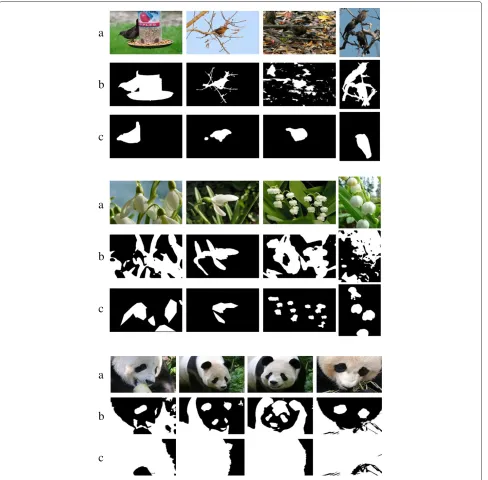
As illustrated in Table 2 and Figure 5, our method out-performs the three methods in terms of segmentation accuracy as well as computation time. The method of Joulin et al. [19] takes superpixels as basic units, thus the objects’ boundaries are not clearly delineated as some superpixels merge foreground and background regions together. CoSand [4] only focuses on extracting the large coherent regions, it performs poorly for the figure-ground separation task. For example, it only extracts the black regions in the panda image set, failing to detect the white regions as foreground objects. ClassCut [9] can extract most of foreground regions, while it tends to omit some fragile regions like the petals in the Oxford flowers dataset. This is because the over-segmentation method it

Table 2 The segmentation performance of CoSand [4], ClassCut [9], Joulin et al. [19] and our method over the Oxford flowers, UCSD birds and CMU iCoseg datasets

Oxford flowers UCSD birds CMU iCoseg

Method Accuracy Time(s) Accuracy Time(s) Accuracy Time(s)

CoSand [4] 0.68 39.21 0.42 37.50 0.52 23.90

ClassCut [9] 0.72 95.96 0.32 93.71 0.51 78.43

Joulin et al. [19] 0.70 33.07 0.35 19.44 0.43 19.19

Our method (initial) 0.67 - 0.52 - 0.64

-Our method (final) 0.84 24.14 0.68 13.11 0.74 11.19

Figure 5Segmentation comparison with ClassCut [9], Joulin et al. [19] and CoSand [4] on the Oxford flowers, UCSD birds and CMU iCoseg datasets.The regions in white indicate the foreground objects, while the regions in black stand for the backgrounds.(a)The input images, (b)ClassCut [9]’s results,(c)Joulin et al. [19]’s results,(d)CoSand [4]’s results, and(e)our method’s results.

adopted has merged the boundaries with backgrounds. In contrast, our method can extract the whole foreground object accurately, no matter it is composed of one or several appearance distributions. We attribute this to the initialization scheme and the appearance sharing among images.

UCSD birds and CMU iCoseg datasets, respectively. Figure 6 compares some segmentation results obtained in the initialization and last stages. We can observe that most errors induced in the initialization stage are rectified finally.

5.3.2 Initialization performance

One contribution of our method is applying saliency detection with guided filtering to initially obtain fore-ground regions. To verify this stage’s effectiveness, we compare it with other initialization schemes, including

Figure 6Segmentation results obtained before and after sharing appearance similarity.The white regions denote the foreground objects, while the black regions stand for the backgrounds.(a)The input images,(b)the segmentation results obtained in the initial stage, and

Table 3 The segmentation performance obtained by the initial stages of BiCos [18], CoSand [4], ClassCut [9] and our method over the Oxford flowers, UCSD birds and CMU iCoseg datasets

Oxford flowers UCSD birds CMU iCoseg

Method Accuracy Time(s) Accuracy Time(s) Accuracy Time(s)

BiCos [18] 0.72 14.06 0.48 8.40 0.61 7.27

CoSand [4] 0.63 20.00 0.32 12.00 0.43 10.00

ClassCut [9] 0.57 23.32 0.42 18.00 0.31 11.40

Our method 0.67 2.70 0.52 1.55 0.64 1.32

The values in bold indicate the best results.

GrabCut [25] used in BiCos [18], the large coherence regions presented in CoSand [4] and the initialization stage of ClassCut [9]. Since the initialization stages are all performed in still images, we randomly select 100 images from the three datasets for comparison.

In BiCos [18], GrabCut [25] estimates the foreground regions by optimizing a MRF energy function with the foreground and background color models. The fore-ground model is estimated with a bounding box in the center (50 % of the image size) and the background model is estimated from the rest. In CoSand [4], the foreground region comes from K-way segmentation. As suggested in the article, the number of segments K ranges from two to eight and the highest accuracies are reported. In ClassCut [9], a class model with shape, location and color cues is initialized by an object detector [24], and the fore-ground regions are estimated by optimizing a MRF energy function with the class model.

Table 3 shows the average segmentation accuracies as well as computation time for different initializa-tion schemes. As can be seen, our initializainitializa-tion scheme achieves best performance for the UCSD birds and CMU iCoseg datasets, while GrabCut [25] reports higher accuracy than ours for the Oxford flowers dataset. We believe that this is due to the characteristics of the dataset, where the objects tend to be centered in the image and have a good contrast with the back-grounds. Under such constraint situation, the class models can be accurately estimated by GrabCut [25]. In con-trast, the UCSD birds and CMU iCoseg datasets are more general, which verifies that our method is more flexible to be applied to real situations. Besides, our initialization scheme is significantly faster than those competitors.

5.3.3 Running time

One advantage of our method is its efficiency. Table 2 compares the running time of our methods with oth-ers. To further learn about how the time is cost in the whole process, we analyze each step’s performance on the Oxford flowers, UCSD birds and CMU iCoseg datasets. As shown in Table 4, most of the time is spent on extracting superpixels, while the main stages in the arti-cle, including saliency detection, local refinement, global message transferring and heat energy diffusion cost only 8.01 s in total for the Oxford flowers dataset, 4.92 s for the UCSD birds dataset and 4.32 s for the CMU iCoseg dataset.

5.4 Failure cases

Our method works under an assumption that the inter-ested objects should stand out as saliency. Yet such an assumption may not hold in some cases. Figure 7 illus-trates some failure cases of our method for the images from the UCSD birds, Oxford flowers and CMU iCoseg datasets. As illustrated, although the bird, flower, and panda regions recur in the image sets, they are not too distinct with other regions to be detected as saliency. Our method fails to separate them from the backgrounds under such cases.

6 Conclusion

In this article, we present an iterative energy minimization method along a hierarchical graph for object cosegmen-tation. Starting from initialization by saliency detection, the method alternates via updating the latent parameters, refining object segmentation and propagating appearance distribution among images. Experiments demonstrate its superiority over start-of-the-art methods in aspects of

Table 4 The running time cost by each stage of our method over the Oxford flowers, UCSD birds and CMU iCoseg datasets

Dataset Superpixel

extraction

Heat source extraction

Saliency detection

Local refinement

Heat energy transfer and diffusion

Total time (s)

Oxford flowers 16.13 0.28 0.24 2.28 5.21 24.14

UCSD birds 8.19 0.14 0.18 1.47 3.13 13.11

a

b

c

a

b

c

a

b

c

Figure 7Failure cases.(a)The input images,(b)the segmentation results, and(c)the ground truth.

accuracy and computation time. We attribute this to the combination of saliency detection, guided filtering and heat sources.

Still there are several issues remained to be explored. Currently, our method works under the assumption that the input images contain the common foreground objects. It is worth exploring a more general case that the input image set is composed of several groups where each group contains the common foreground objects. In addition, considering the parallelization capacity of our method, the

system can be redesigned for implementation in parallel graphic hardware.

Endnotes

Competing interests

The authors declare that they have no competing interests.

Acknowledgements

This work is supported by the National 863 Program of China under Grant No.2012AA011803, the Specialized Research Fund for the Doctoral Program of Higher Education of China under Grant No.20121102130004 and the Natural Science Foundation of China under Grant No.61170188.

Received: 9 June 2012 Accepted: 2 February 2013 Published: 26 February 2013

References

1. C Rother, V Kolmogorov, T Minka, A Blake, inIEEE Conference on Computer Vision and Pattern Recognition, vol. 1. Cosegmentation of image pairs by histogram matching (Washington, 2006), pp. 993–1000

2. D Batra, A Kowdle, D Parikh, inIEEE Conference on Computer Vision and Pattern Recognition, vol. 1. iCoseg: interactive co-segmentation with intelligent scribble guidance (San Francisco, 2010), pp. 3169–3176 3. S Vicente, V Kolmogorov, C Rother, inEuropean Conference on Computer

Vision, vol. 2. Cosegmentation revisited: models and optimization (Heraklion, 2010), pp. 465–479

4. G Kim, EP Xing, L Fei-Fei, T Kanade, inIEEE International Conference on Computer Vision, vol. 1. Distributed cosegmentation via submodular optimization on anisotropic diffusion (Barcelona, 2011), pp. 169–176 5. B Russell, A Efros, J Sivic, W Freeman, A Zisserman, inIEEE Conference on

Computer Vision and Pattern Recognition, vol. 2. Using multiple segmentations to discover objects and their extent in image collections (New York, 2006), pp. 1605–1614

6. L Cao, L Fei-Fei, inIEEE International Conference on Computer Vision, vol. 1. Spatially coherent latent topic model for concurrent segmentation and classification of objects and scenes (Rio de Janeiro, 2007), pp. 1–8 7. B Zhao, L Fei-Fei, EP Xing, inEuropean Conference on Computer Vision,

vol. 5. Image segmentation with topic random field (Heraklion, 2010), pp. 785–798

8. J Winn, N Jojic, inIEEE International Conference on Computer Vision, vol. 1. LOCUS—learning object classes with unsupervised segmentation (Beijing, 2005), pp. 756–763

9. B Alexe, T Deselaers, V Ferrari, inEuropean Conference on Computer Vision, vol. 5. ClassCut for unsupervised class segmentation (Heraklion, 2010), pp. 380–393

10. H Arora, N Loeff, DA Forsyth, N Ahuja, inIEEE Conference on Computer Vision and Pattern Recognition, vol. 1. Unsupervised segmentation of objects using efficient learning (Minneapolis, 2007), pp. 1–7 11. Y Chen, L Zhu, A Yuille, H Zhang, inIEEE Conference on Computer Vision

and Pattern Recognition, vol. 1. Unsupervised learning of probabilistic object models (POMs) for object classification, segmentation and recognition (Anchorage, 2008), pp. 1–8

12. V Kolmogorov, R Zabih, What energy functions can be minimized via graph cuts. IEEE Trans. Pattern Anal. Mach. Intell.2(26), 147–159 (2004) 13. P Felzenszwalb, Efficient belief propagation for early vision.

Int J. Comput. Vis.70, 41–54 (2006)

14. A Levinshtein, A Stere, KN Kutulakos, DJ Fleet, SJ Dickinson, K Siddiqi, TurboPixels: fast superpixels using geometric flows. IEEE Trans. Pattern Anal. Mach. Intell.31, 2290–2297 (2009)

15. L Grady, Random walks for image segmentation. IEEE Trans. Pattern Anal. Mach. Intell.28, 1768–1783 (2006)

16. K He, J Sun, X Tang, inEuropean Conference on Computer Vision, vol. 1. Guided image filtering (Heraklion, 2010), pp. 1–14

17. M Cheng, G Zhang, NJ Mitra, X Huang, S Hu, inIEEE Conference on Computer Vision and Pattern Recognition, vol. 1. Global contrast based salient region detection (Colorado Springs, 2011), pp. 409–416 18. Y Chai, V Lempitsky, A Zisserman, inIEEE International Conference on

Computer Vision, vol. 1. BiCoS: a bi-level co-segmentation method for image classification (Barcelona, 2011), pp. 2579–2586

19. A Joulin, F Bach, J Ponce, inIEEE Conference on Computer Vision and Pattern Recognition, vol. 1. Discriminative clustering for image co-segmentation (San Francisco, 2010), pp. 1943–1950

20. T Hofmann, Unsupervised learning by probabilistic latent semantic analysis. Mach. Learn.43, 177–196 (2001)

21. J Shi, J Malik, inIEEE Conference on Computer Vision and Pattern Recognition, vol. 1. Normalized cuts and image segmentation, (San Juan, 1997), pp. 731–737

22. L Mukherjee, V Singh, C Dyer, inIEEE Conference on Computer Vision and Pattern Recognition, vol. 1. Half-integrality based algorithms for cosegmentation of images (Miami, 2009), pp. 2028–2035 23. D Hochbaum, V Singh, inIEEE Conference on Computer Vision, vol. 1.

An efficient algorithm for co-segmentation (Kyoto, 2009), pp. 269–276 24. B Alexe, T Deselaers, V Ferrari, inIEEE Conference on Computer Vision and

Pattern Recognition, vol. 1. What is an object (San Francisco, 2010), pp. 73–80

25. C Rother, V Kolmogorov, A Blake, Grabcut—interactive foreground extraction using iterated graph cuts. ACM Trans Graph.

23(3), 309–314 (2004)

26. R Duda, P Hart, D Stork,Pattern classification, 2nd edn. (Wiley Press, New York, 2000)

doi:10.1186/1687-5281-2013-11

Cite this article as:Liet al.:A hierarchical graph model for object coseg-mentation.EURASIP Journal on Image and Video Processing20132013:11.

Submit your manuscript to a

journal and benefi t from:

7Convenient online submission 7Rigorous peer review

7Immediate publication on acceptance 7Open access: articles freely available online 7High visibility within the fi eld

7Retaining the copyright to your article