http://www.sciencepublishinggroup.com/j/acm doi: 10.11648/j.acm.20190803.12
ISSN: 2328-5605 (Print); ISSN: 2328-5613 (Online)
The Application of Bessel Function in the Definite Solution
Problem of Cylindrical Coordinate System
Wenjie He, Meiling Zhao
*School of Mathematics and Physics, North China Electric Power University, Baoding, China
Email address:
*
Corresponding author
To cite this article:
Wenjie He, Meiling Zhao. The Application of Bessel Function in the Definite Solution Problem of Cylindrical Coordinate System. Applied and Computational Mathematics. Vol. 8, No. 3, 2019, pp. 58-64. doi: 10.11648/j.acm.20190803.12
Received: July 12, 2019; Accepted: August 10, 2019; Published: August 23, 2019
Abstract:
The variable separation method is an important method to solve the definite solution problems, especially the definite solution problems of cylinder and sphere regions. This method can solve these problems on cylinder and sphere regions, but the solving procedures are very difficult in the practical application. It is often solved by combining the properties of Bessel functions. In this paper, we propose a method combining Bessel function to solve homogeneous definite solution problem on the cylindrical coordinate system and give the algorithm of solving a definite problem. This algorithm is easy to implement and simplifies the process of calculation. Firstly, the definition and properties of Bessel function are briefly recalled, which are the first and essential step to solve the definite solution problem. Then we give the basic process of solving homogeneous definite solution problem, where consider the problem of the definite solution of the homogeneous wave equation, homogeneous heat conduction equation and Laplace equation. We analyze the solution of the Bessel equation definite solution problem under three kinds of boundary conditions and conclude the algorithm of solving a definite problem. At last, two numerical examples are provided to validate the feasibility of the proposed method.Keywords: Bessel Function, Definite Solution Problems, Cylindrical Coordinate
1. Introduction
Bessel function is one of the most significant special functions, which is widely used in atmospheric science, mechanics, mathematics and other disciplines. Bessel function is obtained when equation Helmholtz and Laplace equation are solved by separating variables in cylindrical or spherical coordinates [12]. There are some limitations to use elementary function to solve the definite problem. Therefore, Bessel functions have been attracted considerable attention. The solution of the definite solution problem usually needs to be converted into the partial differential equation with variable coefficient in cylindrical or spherical coordinate system, then solve by using special functions. There are many classical problems, such as electromagnetic wave propagation waveguides [4, 7], heat conduction problem [1], the vibration mode problem of circular or annular films and so on.
Several special cases of positive integer order of Bessel function were proposed by Swiss mathematician Daniel
function [11].
In this paper, we propose a method combining Bessel function to solve homogeneous definite solution problem of cylindrical coordinate system. The definite solution problems with different boundary conditions are analyzed. A brief outline of this paper is as follows. Section 2 recalls the definition and properties of the Bessel function, which provides a theoretical basis for the following methods. In Section 3, the method of separating variables to solve the homogeneous definite solution problem is summarized, and Bessel equation definite solution problem under three kinds of boundary conditions are analyzed. Numerical examples are provided to validate the proposed method in Section 4. Finally, the paper is concluded.
2. Bessel Function
Bessel function is the solution of Bessel equation, except elementary function. Bessel function is the most commonly used function in mathematics, physics and engineering.
2.1. Bessel Function Definition
Bessel's equation is the equation
2 2 2
'' ' ( ) 0,
x y +xy+ x −v y= (1) where
v
is a constant and is called order of equation, which can be any real number or complex number. The solutions of Bessel's equation are called as Bessel functions, which can be divided into three kinds.The first kind of Bessel functions are often called Bessel functions, which are denoted by J xv( ) and J−v( )x . These can be written in the form
2
0
1 1
( )
! ( 1)
( )
. 2
k v k
v k
x J x
k v k
± ∞
±
=
−
=
Γ ± + +
∑
(2)The second kind of Bessel function are often called Neumann function, which is denoted by Y xv( ). This can be written in the form
cos ( ) ( )
( ) .
sin
v v
v
v J x J
v x
Y x π
π −
−
= (3)
The third kind of Bessel functions often are called Henkel functions, which are denoted by Hv(1)( )x and Hv(2)( )x . These can be written in the form
(1)
(1)
( )
( ) ( ) (
( ) ( ) ,
).
v v v
v v v
H x J x iY
H J iY
x
x x x
= +
= − (4)
(1)
( ) v
H x and Hv( )x ( )x are respectively called the first Henkel function and the second Henkel function.
2.2. Properties of Bessel Function
Bessel functions are characterized by many important properties. Analyzing its properties was the primary step in understanding the Bessel function.
2.2.1. Recursion Formula
Bessel functions have recursive relationships. Taking the first kind of Bessel functions as an example, we have the following recursive formulas
(
)
(
21)
02 2( ) 1( ) ' ( ), ' ( ),
,
( 1) .
m
v v m
v v m
m
v m v m
v v m
xJ x xJ x
x J x J x
d
x J x J
xdx
d
x J x J
xdx x
− −
− − −
+
= =
=
= −
(5)
Similar properties exist in other kind of functions.
2.2.2. Zero Point
The root of J xv( )=0 is called the zero point of J xv( ). ( )
v
J x has an infinite number of individual real zeros in the interval [0, ]∞ , which are distributed symmetrically around the origin on the
x
axis. The zero points of J xv( ) and1( )
v
J+ x are distributed with each other. If
x
is sufficiently large, the distance between the two adjacent zeros of J xv( ) is close toπ
.We know that the zero point of Jv(λ =A) 0 is xn(0) =
λ
nA, then we can obtain the eigenvalues and eigenfunctions,(0)
, 1, 2, , ( ) ( ), 1, 2, .
n n
n v n
x
n A
F x J x n
λ
λ
= =
= =
⋯ ⋯
(6)
2.2.3. Bessel Function Series Expansion
Arbitrary function f x( ) has a continuous first order derivative and the second derivative piecewise continuous in the interval
[ ]
0,A . Suppose f(0) < +∞, ( )f A =0 , then( )
f x must be expanded to the following series
( )
1
( ) ( ),
v n n v n
x
f x C J x
A ∞
=
=
∑
(7)where the zero point of J xv( ) is xn( )v , and
( )
0
( 2 2 )
1
2 (
(
) )
) (
. v A
n
v v n
v n
x xf x J x dx
A C
A J + x
=
∫
(8)3. Solving the Definite Solution Problem
solution of partial differential equations, which is widely used in various definite solution problems. Bessel functions make it easier to solve the definite solution problem in cylindrical coordinate system. We consider the problem of the definite solution of the homogeneous wave equation, homogeneous heat conduction equation and Laplace equation.
3.1. Separating Variables
A set of ordinary differential equations is obtained by separating variables from the original equation.
3.1.1. Laplace Equation
2 2 2
2 2 2 0.
u u u
x y z
∂ +∂ +∂ =
∂ ∂ ∂ (9)
The expression in cylindrical coordinate system is
2 2 2
2 2 2 2
1 1
0.
u u u u
r r
r r θ z
∂ + ∂ + ∂ +∂ =
∂
∂ ∂ ∂ (10) Let the form of variable separation be
( , , ) ( ) ( ) ( ).
u rθ z =R r Φθ Z z (11) Substituting the above equation into (10), we obtain
2
1 1
'' ' '' '' 0.
ZR ZR RZ R Z
r r
Φ + Φ + Φ + Φ = (12)
Multiplying both sides of the equation by
2
r
R ZΦ , we get
2 R R 2Z 2.
r r r v
R R Z
′′+ ′+ ′ = −Φ =
Φ
′ ′′
(13)
It decomposes into two equations 2
''
v
0,
Φ + Φ =
(14)2 2 2
.
R R Z
r r r v
R + R + Z
′′=
′′ ′
(15)
Dividing in both sides of (15) by r2 and transfers, we get
2
2 2
1
, 0.
R R v Z
R +r R −r = − Z = −λ λ
′ ′′
≠
′ ′
(16)
Eventually we can decompose the original equation into
2
2
2 2
2
0,
0, 1
'' ' ( ) 0.
v
Z Z
v
R R R
r r
λ
λ
Φ + Φ =
− =
+
′′ ′′
+ − =
(17)
3.1.2. Homogeneous Wave Equation
2 2 2 2
2
2 2 2 2 0.
u u u u
a
t x y z
∂ − ∂ +∂ +∂ =
∂ ∂ ∂ ∂ (18)
First, we separate time variables from space variables. Supposing that u( , )vt =T t V( ) ( )v , then
2
2 .
T V
k V
a T ∆ = −
′ = ′
(19)
It decomposes into two equations 2 2
''
0,
T
+
k a T
=
(20)2
0.
V k V
∆ + = (21) Using cylindrical coordinates for (21), we treat ( , , ) ( ) ( ) ( )
u rθ z =R r Φθ Z z as a new variable, three equations can be decomposed by the same method. Finally, we can decompose the original equation into
2 2
2
2
2 2 2
2
0, 0, 0, 1
'' ' ( ) 0.
T k a T
v
Z Z
v
R R k R
r r
λ
λ
′′
′′ ′′
+ =
Φ + Φ =
− =
+ + − − =
(22)
3.1.3. Homogeneous Heat Conduction Equation
2 2 2
2
2 2 2 0.
u u u u
a
t x y z
∂ − ∂ +∂ +∂ =
∂ ∂ ∂ ∂ (23)
Similarly, first we separate the time variables, and then we separate the space variables in cylindrical coordinates. We can separate the original equation to get
2 2
2
2
2 2 2
2
0, 0, 0, 1
'' ' ( ) 0.
T k a T
v
Z Z
v
R R k R
r r
λ
λ
+ =
Φ + Φ = − ′
′′
=
+ + − − =
′′
(24)
3.2. Solving the Eigenvalue Problem 3.2.1. General Condition
We consider the general case ''( ) ( ) 0.
X x +ωX x = (25) In the situation of ω<0, the general solution of the equation is
( ) x x.
In the situation of ω=0, the general solution of the equation is
( ) .
X x =Ax+B (27) In the situation of ω>0, the general solution of the equation is
( ) cos sin .
X x = A
ω
x+Bω
x (28) Then the solution sequence Xn( ),x n=1, 2,⋯ is obtainedaccording to the boundary conditions.
3.2.2. Eigenvalue Problems of Bessel Equation
2 2
2
1
( v ) 0, 0.
R R R
r λ r λ
′′+ ′+ − = ≠ (29)
Supposing that x=λr the equation can be reduced to
2 2 2
( ) 0,
xx x
x R +xR + x −v R=
which is
v
order Bessel equation, and the general solution is ( ) v( ) v( ).R r = AJ λr +BY λr (30) Since R(0)< +∞ , B=0 . The above equation can be rewritten as
( ) v( ).
R r =AJ λr (31) Firstly, we consider the first kind of boundary conditions
0
( ) 0, (0)
R r = R < +∞, we obtain A≠0 and Jv(λr0)=0. In other words, we need to find the zero point of J xv( )=0.
Let xn( )v represents the n-th positive root of J xv( )=0,
( )
0 ( )
, 1, 2, . v nv
n
x n r
λ = = ⋯
The solution sequence for
( ) ( ), 1, 2, .
n v n
R r =J λ r n= ⋯ (32)
Next, we consider the second kind of boundary conditions
0
( ) 0, (0)
R r′ = R < +∞.
0
0
( ) ( ) 0,
v v
r r d
J r J r
dr λ = =λ ′ λ = (33) from R r( )0 =0 and
( ) ( )
0
, 1, 2, v
v n
n
x n r
λ = = ⋯
where x( )nv means the n-th zero of J xv′( )=0.
Finally, from the third kind of boundary conditions
0 0
( ) '( ) 0, (0)
R r +CR r = R < +∞, we have
0 0
( ) ( ) 0.
v v
J r C J r
λ ′ λ + λ ′ λ = (34) According to the properties of Bessel function, the above equation can be rewritten as
0
0 1 0
0
( ) ( ).
v v
r
J r J r
r v C
λ
λ = + λ
+
(35)
Then
( ) ( )
0
, 1, 2, v
v n
n
x n r
λ = = ⋯
where xn( )v means the n-th zero of (35).
3.3. Superposing Solution Sequences
From the above process, the formal solution can be obtained according to the principle of superposition
( , , , ) ( , , , )
( ) ( ) ( ) ( ). n
n n n t
u r z t u r z t
R r Z zT t
θ
θ
θ
=∑
=∑ Φ (36)
Then we confirm the correlation coefficient according to the initial conditions. Finally, we solved the definite solution problem.
Consequently, we give an algorithm of solving a definite problem as following.
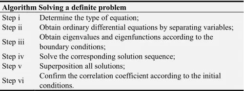
Table 1. The algorithm of solving a definite problem.
Algorithm Solving a definite problem
Step i Determine the type of equation;
Step ii Obtain ordinary differential equations by separating variables;
Step iii Obtain eigenvalues and eigenfunctions according to the boundary conditions;
Step iv Solve the corresponding solution sequence; Step v Superposition all solutions;
Step vi Confirm the correlation coefficient according to the initial conditions.
4. Numerical Example
In this section, we present numerical examples to illustrate our methods in the above sections.
Example 1 Consider the axisymmetric free vibration problem of an infinitely long cylinder with radius r0 =0.5.
2
0
0.5
2 0
0
, ,
. 0,
0, 1 4 tt
r
r
t
t
u a u
u u
r
u
u r
t
=
=
=
=
= ∆ ∂
< +∞ =
∂ ∂
= = −
∂
(37)
Suppose that the vibrational displacement of the particle is ( , , , )
( )
,( ) ( )
u r t =R r T t .We can separate the original equation to get
( )
2 2( )
0,
T′′ t +
λ
a T t = (38)( )
1( )
( )
0.
R r R r R r
r +λ
′′ + ′ = (39)
The solution of (38) is
( )
cos(
)
sin(
)
, 1, 2, .n n n n n
T t =A a
λ
t +B aλ
t n= ⋯ (40)Equation (39) is Bessel function of order v=0, its general solution is
( )
0( )
0( )
.R r =CJ
λ
r +DYλ
r (41) This boundary belongs to the second boundary condition, we haveD=0, the eigenvalues and eigenfunctions of Bessel equation are(0)
0
0
, 1, 2, , ( ) ( ), 1, 2, ,
n n
n n
x
n r
R r J r n
λ
λ
= =
= =
⋯ ⋯
where x(0)n is the zero point of J x0′( ).
According to the principle of linear superposition, the general solution of original solution can be expressed as
1
0 1
( , ) ( ) ( )
cos( ) sin( ) ( ),
n n
n
n n n n n
n
u r t R r T t
A aλ t B aλ t J λ r
∞
= ∞
=
=
= +
∑
∑
(42)
where coefficients An and Bn are determined by initial condition
0 1
2 0
1
( ) 0,
4 . ( ) 1
n n
n
n n n
n
A J r
B a J r r
λ
λ λ
∞
= ∞
=
=
= −
∑
∑
(43)
Then we can solve
0.5 2
0 2
1 0
1 2
0 2
1 0
2 3 2
1
0,
1 8
(1 4 ) ( ) (0.5 )
2
(1 ) (0.5 )
(0.5 ) 16 0.5
,
0.5 1, 2, .
( )
( )
n
n n
n n
n
n n
n
n n
A
B r r J r dr
a J
t t J t dt
a J
J
a J
n
λ
λ λ
λ
λ λ
λ
λ λ
=
= −
= −
=
=
∫
∫
⋯
Substituting the coefficient into equation (44), we have
2
0 3 2
1 1
(0.5 ) 16
( , ) ( ) sin
.5 ) ( )
0
( .
n
n n
n n
n
J
u r t J r a t
a J
λ
λ
λ
λ
λ
∞
=
=
∑
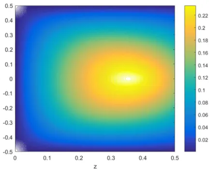
(44)The vibration displacement of cylinder is given by computer simulation, see Figures 1-3.
Figure 1. The vibration displacement of cylinder with a=1.
Figure 2. The vibration displacement of cylinder with a=2.
Example 2 There is an empty cylinder with a conductor wall. The height of the cylinder is h=1, the radius is r0 =1, the top of the cylinder potential is 0.2, the side and the decisive potential are 0. Below we solve the potential distribution inside the cylinder.
Using cylindrical coordinate system, we can find that the conditions of the solution are independent of the angle θ and only related to ,r z. The problem can be boiled down to the following definite problem.
2 2
2 2
1 0
0 1
1
0,
0, ,
0, 0.2.
r r
z z
u u u
r r
r z
u u
u u
= =
= =
∂ + ∂ +∂ =
∂
∂ ∂
= < +∞
= =
(45)
We use the separation of variables method to solve the above problems. Suppose that u r z
( )
, =R r Z z( ) ( )
, we can separate the original equation to obtain''( ) ( ) 0,
Z z −λZ z = (46)
2 2 2
''( ) ( ) ( ) 0.
r R r +rR r +
λ
r R x = (47) The solution of (46) is( ) nz nz, 1, 2, .
n n n
Z z =A eλ +B e−λ n= ⋯ (48)
Equation (47) is Bessel function of order v=0, its general solution is
0 0
( ) ( ) ( ).
R r =CJ λr +DY λr (49) This boundary belongs to the first boundary condition, we have D=0, the eigenvalues and eigenfunctions of Bessel equation are
(0)
0
0
, 1, 2, , ( ) ( ), 1, 2, ,
n n
n n
x
n r
R r J r n
λ
λ
= =
= =
⋯ ⋯
where x(0)n is the zero point of J x0( ).
According to the principle of linear superposition, the general solution of original solution can be expressed as
1
0 1
( , ) ( ) ( )
[ n n ] ( ),
n n
n
z z
n n n
n
u r z R r Z z
A eλ B e λ J λ r
∞
= ∞
−
=
=
= +
∑
∑
(50)
where coefficients An and Bn are determined by initial conditions,
0 1
0 1
( ) ( ) 0,
[ n n] ( ) 0.2.
n n n
n
n n n
n
A B J r
A eλ B e λ J r
λ
λ ∞
= ∞
−
=
+ =
+ =
∑
∑
(51)
Simplifying the above equations, we have
1 0 0
2 1
1
0,
0.4 ( )
( ) 0.4 .
( )
n n
n n
n
n n
n
n n
A B
rJ r dr
A e B e
J
J
λ λ λ
λ
λ λ
−
+ =
+ =
=
∫
Finally, the coefficients are
1
0.2 . sinh ( )
n n
n n n
A B
J
λ λ λ
= − =
Substituting the coefficients into (50), we obtain
0 1
1
0.4
( , ) sinh( ) ( ).
sinh ( ) n n
n n n
n
u r z z J r
J
λ
λ
λ
λ
λ
∞
=
=
∑
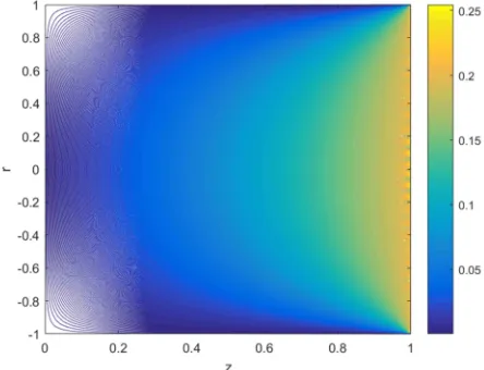
(52)Figure 4 shows the potential distribution inside the cylinder.
Figure 4. The potential distribution inside the cylinder.
5. Conclusion
Acknowledgements
This research was supported by the Fundamental Research Funds for the Central Universities (No. 2018MS129).
References
[1] A. Mitchell, R. Pearce, Explicit difference methods for solving the cylindrical heat conduction equation. Mathematics of Computation, 1963, vol. 17, no. 84, pp. 426-432.
[2] C. Rossetti, Approximate expressions for the Bessel functions and their zeros. Nuovo Cimento B, 1987, vol. 100, no. 4, pp. 515–536.
[3] E. Karatsuba. Fast evaluation of Bessel functions. Integral Transforms and Special Functions, 1993, vol. 1, no. 4, pp. 269-276.
[4] H. Bateman, The solution of the wave equation by means of definite integrals. Bulletin of the American Mathematical Society, 1918, vol. 24, no. 6, pp. 296-301.
[5] J. Harrison, Fast and accurate Bessel function computation. Proceedings of the 19th IEEE international symposium on computer arithmetic, 2009, pp. 104-113.
[6] M. Higgins, A theory of the origin of microseisms. Philosophical Transactions of the Royal Society A: Mathematical, Physical and Engineering Sciences, 1950, vol. 243, no. 857, pp. 1-35.
[7] R. Higdon, Numerical absorbing boundary conditions for the wave equation. Mathematics of Computation, 1987, vol. 49, no. 179, pp. 65-90.
[8] S. Liu, S. Liu, Special function. Meteorological press, 1988. [9] S. Zhou, S. Zhang, S. Sun, Special function applied in
mechanical analysis. Journal of Shandong University of Technology, 1994, vol. 4, pp. 306-311.
[10] T. Zhan, Inquiring into fixed answers to the thermal transmission equation. Journal of Dalian university, 1998, vol. 2, pp. 34-37.
[11] W. Cheng, Application of Bessel functions in solving parabolic partial differential equations. Mathematics Learning and Research: Teaching Research Edition, 2017, vol. 14, pp. 9-10.
[12] Y. Taitel, On the parabolic, hyperbolic and discrete formulation of the heat conduction equation. International Journal of Heat and Mass Transfer, 1972, vol. 15, no. 2, pp. 369-371.
[13] Z. Wang, D. Guo, Introduction to special functions. Science press, 1965.
[14] H. Wang, A general solution to the common eigenvalue problem, Journal of Qingdao University of Science and Technology, 2018, vol. 39, no. 1, pp. 134-138.
[15] K. Parand, M. Nikarya, Application of Bessel functions and Jacobian free Newton method to solve time-fractional Burger equation, Nonlinear Engineering, 2019, vol. 8, pp. 688-694. [16] R. Gauthier, A. Mohammed, Cylindrical space fourier-Bessel