Evaluating the effect of Japan’s 2004 postgraduate training programme on the spatial distribution of physicians

(1)

R E S E A R C H

Open Access

Evaluating the effect of Japan

’

s 2004 postgraduate

training programme on the spatial distribution of

physicians

Rie Sakai

1,2,3*

, Hiroshi Tamura

4,5

, Rei Goto

6,7

and Ichiro Kawachi

1

Abstract

Background:In 2004, the Japanese government permitted medical graduates for the first time to choose their training location directly through a national matching system. While the reform has had a major impact on physicians’ placement, research on the impact of the new system on physician distribution in Japan has been limited. In this study, we sought to examine the determinants of physicians’practice location choice, as well as factors influencing their geographic distribution before and after the launch of Japan’s 2004 postgraduate medical training programme. Methods:We analyzed secondary data. The dependent variable was the change in physician supply at the secondary tier of medical care in Japan, a level which is roughly comparable to a Hospital Service Area in the US. Physicians were categorized into two groups according to the institutions where they practiced; specifically, hospitals and clinics. We considered the following predictors of physician supply: ratio of physicians per 1,000 population (physician density), age-adjusted mortality, as well as measures of residential quality. Ordinary least-squares regression models were used to estimate the associations. A coefficient equality test was performed to examine differences in predictors before and after 2004.

Results:Baseline physician density showed a positive association with the change in physician supply after the launch of the 2004 programme (P-value < .001), whereas no such effect was found before 2004. Urban locations were inversely associated with the change in physician supply before 2004 (P-value = .026), whereas a positive association was found after 2004 (P-value < .001). Urban location and area-level socioeconomic status were positively correlated with the change in hospital physician supply after 2004 (P-values < .001 for urban centre, and .025 for area-level socioeconomic status), even though in the period prior to the 2004 training scheme, urban location was inversely associated with the change in physician supply (P-value = .015) and area-level socioeconomic status was not correlated.

Conclusion:Following the introduction of the 2004 postgraduate training programme, physicians in Japan were more likely to move to areas with already high physician density and urban locations. These changes worsened regional inequality in physician supply, particularly hospital doctors.

Keywords:Human resources, Physician distribution, Postgraduate medical training programme, Japan

* Correspondence:[email protected] 1

Department of Social and Behavioural Sciences, Harvard School of Public Health, 677 Huntington Avenue, Boston, MA 02215, USA

2

Department of Medical Education, Juntendo University School of Medicine, Hongo 2-1-1 Bunkyo-ku, Tokyo, Japan

Full list of author information is available at the end of the article

(2)

Background

Optimizing physician supply and distribution are vital in-gredients of sustaining equitable access to essential health services. However, there may be a tension between expanding access to physician supply versus improving the quality of their training, as our case study from Japan will illustrate.

In 2004, the Japanese Ministry of Health, Labour and Welfare (MHLW) sought to improve the quality of medical residency training nationwide by instituting a new post-graduate medical education (PGME) programme [1]. Prior to 2004, medical graduates commenced their specialty training immediately after graduating from medical school. Since medical graduates ended up being trained only in their chosen specialty, they had little or no experience in other fields. Since 2004, a 2-year general residency has been required of all medical graduates, ensuring that residents rotate through different specialties to gain hands-on experience at teaching hospitals designated by MHLW. These hospitals would include both university-affiliated and non-university-university-affiliated hospitals, encom-passing both public and private institutions [2]. After 2004, new physicians commenced their specialty train-ing followtrain-ing the mandatory 2-year residency traintrain-ing programme.

Before 2004, a majority of new graduates entered their specialty training programme at the university hospital associated with the medical school where they graduated. In those times, physicians were dispatched to non-university hospitals by the department of their specialization in the university hospital, and individual choice was not considered.

As part of the 2004 reforms, the Ministry permitted medical graduates to choose their preferred residency loca-tion directly through a naloca-tional matching system for the first time [2]. Then, medical graduates tended to select in-dependent urban hospitals not affiliated with a university for their training rather than university hospitals [3,4]. Even though the matching system only applied to the 2-year residency training programme, young physicians now had the freedom to choose a residency location that could also provide them the specialty training, in terms of targeted mentors and professional recognition, when the residency was completed. As a result, young physicians tended to stay at the same location and continue their specialty train-ing after the residency traintrain-ing. Subsequently, the number of incoming physicians at university hospitals decreased. Medical specialty departments in university (teaching) hospitals normally dispatch physicians at all levels to other affiliated hospitals. Because the number of physicians at university hospitals has decreased, university hospitals find it increasingly difficult to send physicians to affiliated hospitals, which are often located in rural and underserved areas [5]. Furthermore, physicians working in rural areas

return to university hospitals to fill the void left by the lack of new medical graduates. The Japan Medical Association Research Institute reported that almost 60% of all uni-versity hospitals have reduced the dispatch of physicians to other medical institutions since the launch of the new training programme [6].

To determine if the 2004 reform had the unintended consequence of impacting physician supply and distribu-tion, we performed an ecological analysis using nationally available data.

In a previous study, we examined the impact of the 2004 reform on the supply of paediatricians in Japan [7]. Our previous study suggested that the 2004 medical residency scheme had the unintended consequence of making it easier for new graduates to choose residency training location, exacerbating regional inequalities in paediatri-cian supply. A limitation of our previous study was that we ignored the distinction between hospital-based clinicians and smaller-clinic-based physicians (that is primary care clinics with fewer than 20 beds). The 2004 reforms affected resident training programmes that take place primarily in training hospitals designated by the MHLW, as opposed to physicians’ practice locations in small clinics. Therefore, the spatial distribution for clinic-based physicians would not be expected to be affected by the new scheme.

Indeed Toyabe [8] analyzed the time trends in the number and distribution of physicians between 1996 and 2006 and showed that the increasing inequality in geographic distribu-tion of hospital-based clinicians was markedly worse com-pared to clinic-based physicians; moreover, the number of physicians working at hospitals increased over time in urban areas but not in areas with low population density.

In this study, we sought to disaggregate the hospital clinician trends from clinic-based physicians. We are interested in 2 questions: first, what are the principal drivers of physicians’practice location choice, and second, what factors affected physician distribution before and after the launch of the new programme in 2004?

Data and methods

Unit of analysis

(3)

transportation, and geography, and are roughly comparable to Hospital Service Areas in the US. STMs are considered independent administrative areas from a health service per-spective, and are less prone to local spillovers compared to municipalities or counties (typically used in other studies) [8-14]. The total number of STMs did not change signifi-cantly during the study period, which was between 1998 and 2010, although borders were redrawn. The STM boundaries from 2010 (n = 346) were used in this study.

Data

Dependent variable

Our main dependent variables of interest are differences in numbers of physicians between the 2 4-year time periods: 1998 to 2002, which represents the period before the 2004 programme started (pre-period), and 2006 to 2010, which represents the period after the introduction of the 2004 programme (post-period). That is to say, the results can be interpreted as such: when the estimates are negative, the predictors are related to decreases in the number of physi-cians. When the estimates are positive, the predictors are related to increases in the number of physicians.

Only physicians who mainly worked as health care ser-vice providers are included, while physicians who were engaged in basic research or government service were excluded from the analysis. Physicians were categorized into two groups according to the institutions where they practiced: hospitals versus clinics.

Independent variables

The two main predictors of interest for the change in physician supply analysis were: measures of need and mea-sures of residential quality, as generally highlighted in the literature on physicians’ practice location choice [15-18]. The 2 primary markers of need that we used were: physi-cians per 1,000 population (physician density), and age-adjusted mortality rates at the beginning of the 2 periods.

We considered urban/rural status as an indicator of residential quality. Municipalities were divided into five categories, based on the metropolitan area code defined by the Ministry of Internal Affairs and Communications: 1) central cities of major metropolitan areas, 2) central cit-ies of metropolitan areas, 3) surrounding municipalitcit-ies of central cities of major metropolitan areas, 4) surrounding municipalities of central cities of metropolitan areas, and 5) other municipalities. This classification is revised, based on the results of the national census in Japan, which is conducted every 5 years.

The classification from 2000 and 2005 (aligned to census years) was used to characterize the pre-period (1998 to 2002) andpost-period(2006 to 2010), respectively. In this study, the metropolitan and the major metropolitan areas were combined into a single category, since there were only 5 central cities among 1,750 municipalities in 2000

and 6 in 2005. This resulted in 3 basic groups: 1) STMs that included central cities for major metropolitan areas and metropolitan areas, defined as urban centres (n = 26 in pre-period and n = 28 in post-period); 2) STMs that include surrounding municipalities of central cities of the metropolitan areas and the major metropolitan areas, which are defined as suburban areas (n = 127 inpre-period

and n = 130 in post-period); and 3) others, which are defined as rural (n = 193 in pre-period and n = 188 in

post-period).‘Rural’ is used as a reference group in the models. Because no standard definition of the term

‘rural’ exists [19-22], we checked the robustness of the model with respect to alternative urban/rural measures. Previous studies have employed one of the following definitions [19]: 1) metropolitan statistical area [10,21], which is comparable to metropolitan area codes in Japan; 2) population size [12,19,21]; and 3) population density [19,23]. We employed population density as an alternative way to define urban/rural status. Under this alternative definition, the STMs with a population density of more than 1,000/km2are defined as urban (n = 68 inpre-period

and n = 67 inpost-period), and the remaining are defined as rural (n = 278 inpre-periodand n = 279 inpost-period). As an additional measure of local residential quality, we also included a composite area-based index of socio-economic status (SES composite index), which was created from indicators representing education, occu-pation, and income. The index was derived from a fac-tor analysis of the percentage of the local population with a college-level education, the percentage of white-collar workers, the unemployment rate, andper capita in-come. Factor scores, formulated by a principal component analysis with varimax rotation, were used to construct a composite index to represent each aspect of SES for the study units [24].

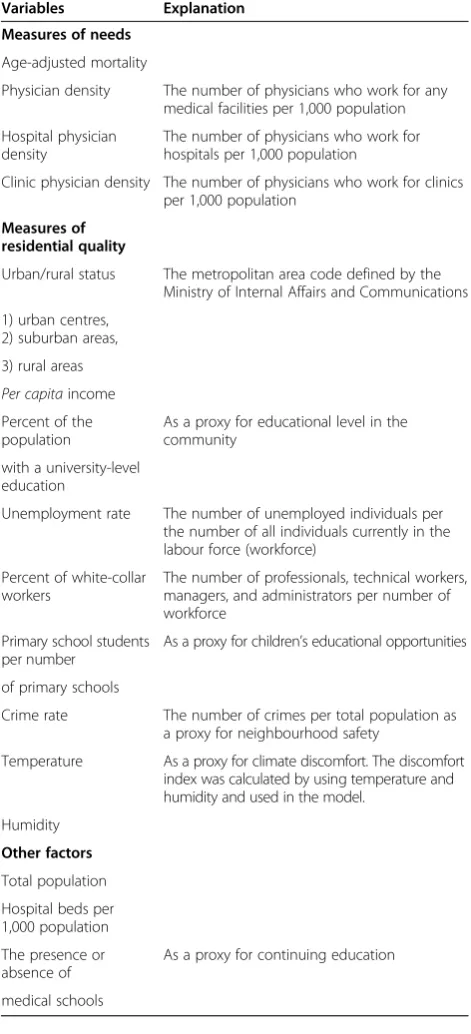
Table 1 describes each of the variables selected in the models. In addition to measures of local need and residen-tial quality, we considered measures of professional inter-actions because the published literature has suggested that professional interactions were important factors that affect physicians’ decisions regarding their practice locations [15-18]. Meteorological data on average temperature and humidity were available only at the prefecture level.

Data sources

(4)

Registers [27] and was used to calculate physician-to-population ratios.

Factors previously shown to be associated with physician supply [15-18] were obtained from publicly-available sec-ondary data. Numbers of deaths by age group of 5-year-olds were obtained from the vital registration system [28-31]. The oldest data yielded mortality dates back to 1999, so the age-adjusted mortality of 1999 was applied in the analysis of the period 1998 to 2002. The

age-adjusted mortality from 2006 was used in the analysis of the period 2006 to 2010. For the calculation of age-adjusted mortality, direct age-standardization was applied using the 1985 model population of Japan as the standard.

The data for the following five variables were obtained from theRegional Statistics by Municipalities, which were produced by the Ministry of Internal Affairs and Commu-nications (MIAC) [32]: 1)per capitaincome; 2) number of hospital beds; 3) number of primary schools; 4) number of primary school students; and 5) crime rates, defined as number of crimes per 1,000 population. The data for the following 4 variables were obtained from the 2000 and 2005 Japanese Census [33-35]: 1) metropolitan area codes; 2) percentage of the population with a college-level education; 3) unemployment rate; and 4) percentage of white-collar workers. Unemployment rates and the percentage of white-collar workers were calculated using the mean of 1995 and 2000 data and applied to the time period 1998 to 2002. Corresponding data from 2005 were applied to analysis of the time period 2006 to 2010. The percentage of the population with a college-level education is only collected every 10 years. The data from 1990 were no longer publicly available. Therefore, data from 2000 were applied to the time period 1998 to2002. The mean of 2000 and 2010 data were applied to the time period 2006 to 2010.

To assess average climate (as a potential factor in physician location preference), the discomfort index, developed by the US Weather Bureau (currently the National Weather Service) and widely used in previous studies [36,37], was calculated by using temperature and humidity. Temperature and humidity could only be ob-tained at the prefecture level; data for the model were retrieved from Regional Statistics by Prefectures, which was produced by MIAC [38].

Statistical analysis

Descriptive statistics of all continuous variables were presented as means with standard deviations and 95% confidence intervals (CIs) for the periods 1998 to 2002 (pre-period) and 2006 to 2010 (post-period). Mean equality tests were performed to examine the statistical significance of the observed differences.

Ordinary least-squares regression models were used to analyze changes in STM-level physician supply in thepre -and post-period. For both periods, changes in physician supply were evaluated as a function of STM-level baseline factors, which were defined as 1998 conditions for the

pre-periodand 2006 conditions for thepost-period. A test of coefficient equality in regressions was performed to examine significant differences in coefficients between the

pre- and thepost-period.

To examine if the main predictors of interest had mean-ingful effects on the change in physician supply, after Table 1 Variables selected in the models

Variables Explanation

Measures of needs

Age-adjusted mortality

Physician density The number of physicians who work for any medical facilities per 1,000 population

Hospital physician density

The number of physicians who work for hospitals per 1,000 population

Clinic physician density The number of physicians who work for clinics per 1,000 population

Measures of residential quality

Urban/rural status The metropolitan area code defined by the Ministry of Internal Affairs and Communications

1) urban centres, 2) suburban areas,

3) rural areas Per capitaincome Percent of the population

As a proxy for educational level in the community

with a university-level education

Unemployment rate The number of unemployed individuals per the number of all individuals currently in the labour force (workforce)

Percent of white-collar workers

The number of professionals, technical workers, managers, and administrators per number of workforce

Primary school students per number

As a proxy for children’s educational opportunities

of primary schools

Crime rate The number of crimes per total population as a proxy for neighbourhood safety

Temperature As a proxy for climate discomfort. The discomfort index was calculated by using temperature and humidity and used in the model.

Humidity

Other factors

Total population

Hospital beds per 1,000 population

The presence or absence of

As a proxy for continuing education

(5)

accounting for the effects of the control variables, likeli-hood ratio tests (LRTs) were performed to compare the models that only included control variables with the ones that included each main predictor of interest or all of these predictors together with the control variables. By doing these LRTs, we can check whether each and all of the predictors have a significant contribution to the ex-planation of changes in physician supply in the pre-or

post-period, that could not already be accounted for by the control variables.

As a robustness check, the under-5-year-old population and the over-65-year-old population were used to calcu-late physician density, because these age groups tend to-wards greater demand for medical services [15].

A two-tailed P-value of less than .05 was considered statistically significant. All analyses were performed using SAS 9.2 software (SAS Institute, Inc., Cary, NC, USA). This study does not directly involve the use of human subjects, nor their identifiable data, but aggregated and de-identified data that was released by the Japanese gov-ernment and is publicly-available. The study was consist-ent with the Declaration of Helsinki.

Results

Table 2 shows the aggregate level change in physician supply. Both the absolute number of physicians and the physician-to-population ratio increased in both the pre -andpost-periods.

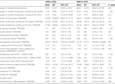
Table 3 shows descriptive statistics of dependent vari-ables, which are differences in numbers of physicians between both 4-year time periods: 1998 to 2002 for the

pre-period, and 2006 to 2010 for the post-period, and continuous independent variables for thepre- andpost

-periods, along with the P-value resulting from testing the Equality of Means. Overall physician density in-creased (P-values for overall physician density was .001, for hospital physician density was .011, and for clinic physician density was < .0001). Table 4 shows descriptive statistics of categorical independent variables for the pre -and post-periods. The number of urban, suburban, and

rural centres changed slightly between the pre-and post-period, and the number of medical schools did not change during the study period.

Table 5 presents the results of our main predictors of interest from the multivariate ordinary least-squares re-gression models controlled by all other factors shown in Table 1 for all physicians. While the change in physician supply was not associated with baseline physician density in thepre-period, it was positively associated with baseline physician density in the post-period(P-value < .0001). In other words, in the post-2004 period, areas with already high physician supply attracted even more physicians. After adjustment for all other variables, we estimated that each unit increase in physician density (1 physician per 1,000 population) in 2006 was associated with an increase in the number of physicians of 64.80 in 2010. While the change in physician supply was inversely associated with urban centres in the pre-period (P-value .026), it was positively associated with urban centres in thepost-period

(P-value < .0001). On average, we estimated that urban centres lost 26.71 physicians from 1998 to 2002 and gained 68.81 from 2006 to 2010, compared to rural areas after adjustment for all other variables.

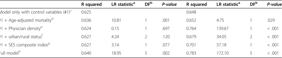
Table 6 shows the results from the LRT for all physi-cians. Physician density, urban/rural status, and the SES composite index did not have meaningful effects on the change in physician supply in thepre-period, while they had significant effects in thepost-period.

Table 7 shows the results from the multivariate ordin-ary least-squares regression analyses for hospital-based clinicians. While the change in hospital physician supply was inversely associated with baseline hospital physician density in the pre-period (P-value = .047), it was posi-tively associated with baseline hospital physician density in thepost-period(P-value < .001). Urban centres and the SES composite index showed statistically-positive associa-tions with the change in hospital physician supply in the

post-period (P-values < .001 for urban centres, and .025 for SES c index), whereas the change in hospital physician supply was inversely associated with urban centres and no

Table 2 The aggregate level change in physician supply at the national level

1998 2002 4-year relative change

(2002 to 1998)/1998

2006 2010 4-year relative change

(2010 to 2006)/2006

Number of all physicians (A = B + C) 236,933 249,574 5.34% 263,540 280,431 6.41%

Number of physicians working at the hospitals (B) 153,100 159,131 3.94% 168,327 180,966 7.51%

Number of physicians working at the clinics (C) 83,833 90,443 7.88% 95,213 99,465 4.47%

Population (millions) (D) 125.57 126.46 0.71% 127.06 127.06 0.00%

Physician densitya_(A/D) _1.89 _1.97 _4.60% _2.07 _2.21 _6.41%

Hospital physician densityb_(B/D) _1.22 _1.26 _3.21% _1.32 _1.42 _7.51%

Clinic physician densityc_(C/D) _0.67 _0.72 _7.13% _0.75 _0.78 _4.46%

a

Number of all physicians per 1,000 population.

b

Number of physicians working at hospitals per 1,000 population.

c

(6)

such effects of SES composite index during thepre-period

(P-value = .015 for urban centres and .483 for SES composite index). The coefficient equality test showed significant differ-ences in coefficients between thepre-periodandpost-period

both for urban centres (P-value < .0001) and the SES composite index (P-value = .026).

Table 8 shows the results from the LRT for physicians working at the hospitals. Hospital physician density and urban/rural status had meaningful effects on the change in hospital physician supply both in the pre- and post

-periods. However, both estimates were negative in the

pre-period, and positive in the post-period. Therefore, Table 3 Descriptive statistics of all dependent and continuous independent variables, the secondary tier of medical care as a unit of analysis (n = 346) The numbers after each variable name indicate the years used in the analyses

1998 to 2002 2006 to 2010

Mean SDa _{95% CIs}b _Mean _SDa _{95% CIs}b

P -valuec

Changes in number of all physicians 36.53 62.10 [29.97 to 43.1] 48.82 120.76 [36.05 to 61.59] .093

Changes in number of physicians working at the hospital 17.43 38.98 [13.31 to 21.55] 36.53 93.92 [26.6 to 46.46] < .001

Changes in number of physicians working at the clinics 19.10 35.83 [15.32 to 22.89] 12.29 35.07 [8.58 to 16.00] .012

Number of all physicians 1998/2006 703.00 1,000.90 [628.3 to 777.7] 786.10 1,144.90 [700.6 to 871.5] .151

Number of physicians working at the hospital 1998/2006 451.20 670.90 [401.1 to 501.3] 504.80 770.70 [447.2 to 562.3] .168

Number of physicians working at the clinic 1998/2006 251.80 346.80 [226.0 to 277.7] 281.30 390.70 [252.2 to 310.5] .138

Age-adjusted mortality 1999/2006 1.15 0.07 [1.15 to 1.16] 0.99 0.06 [0.99 to 1.00] < .001

Physician densityd1998/2006 1.70 0.80 [1.64 to 1.76] 1.85 0.85 [1.78 to 1.91] .001

Hospital physician densitye1998/2006 1.07 0.63 [1.03 to 1.12] 1.16 0.68 [1.11 to 1.12] .011

Clinic physician densityf1998/2006 0.63 0.22 [0.61 to 0.64] 0.68 0.23 [0.67 to 0.70] < .001

Total population (thousands) 1998/2006 364.20 399.50 [334.40 to 394.00] 367.20 417.70 [336.00 to 398.40] .891 Per capitaincome (thousands)g1998/2006 11.75 3.31 [11.51 to 12] 11.36 3.15 [11.12 to 11.59] .023 Percent of the population with a college-level

education 2000/((2000 + 2010)/2)h 10.81 5.25 [10.26 to 11.37] 11.92 5.39 [11.35 to 12.49] .006

Unemployment rate ((1995 + 2000)/2)i_/2005 _4.06 _1.19 _{[3.93 to 4.18]} _5.78 _1.50 _{[5.63 to 5.94]} _{< .001}

Percent of white-collar workers ((1995 + 2000)/2)i_/2005 _14.42 _2.40 _{[14.17 to 14.68]} _13.96 _2.25 _{[13.73 to 14.2]} _.010

Socioeconomic status (SES) composite indexj

−0.02 1.02 [₋0.13 to 0.09] 0.02 0.98 [₋0.08 to 0.12] .593 Number of primary students/school 1998/2006 281.20 133.00 [271.3 to 291.1] 274.00 138.80 [263.7 to 284.4] .325

Crime rate 1998/2006 1.47 0.73 [1.42 to 1.52] 1.10 0.53 [1.06 to 1.14] < .001

Temperature (°C) 1998/2006 15.82 2.53 [15.3 to 16.34] 15.59 2.36 [15.10 to 16.07] .517

Humidity (%) 1998/2006 70.28 4.70 [69.31 to 71.25] 69.44 4.36 [68.54 to 70.33] .205

Discomfort indexk _60.05 _3.87 _{[59.25 to 60.84]} _59.68 _3.58 _{[58.94 to 60.41]} _.500

Hospital beds per 1,000 population 1998/2006 13.89 4.75 [13.54 to 14.24] 13.89 4.62 [13.55 to 14.24] .990

a

Standard deviation.

b

Confidence intervals.

c_P

-value of mean equality test.

d

Number of all physicians per 1,000 population.

e

Number of physicians working at hospitals per 1,000 population.

f

Number of physicians working at health care facilities per 1,000 population.

g

Japanese yen was converted into US$ using the rate that applied in March 2013 of approximately 95 Japanese yen per US$.

h

The percent of college-level education is only collected every 10 years. Data from 2000 were applied to the time period 1998 to 2002, and the mean of 2000 and 2010 data were applied to the time period 2006 to 2010.

i

Unemployment rates and the percentage of white-collar workers were calculated using the mean of 1995 and 2000 data and applied to the time period 1998 to2002.

j

A composite index of socioeconomic indicators created from the percent of the population with a college-level education, percent of white-collar workers, the unemployment rate, andper capitaincome.

k

Calculated by using temperature and humidity.

Table 4 Descriptive statistics of categorical independent variables, the secondary tier of medical care as a unit of analysis (n = 346)

1998 to 2002 2006 to 2010 P-value

n (%) n (%)

Urban centre 26 (7.5) 28 (8.1) 0.677

Suburban 127 (36.7) 130 (37.6)

Rural 193 (55.8) 188 (54.3)

STMa_{s with at least one} medical school

65 (18.79) 65 (18.79) 1.000

a

(7)

the effects of those variables were meaningful in both periods in an opposite direction. SES composite index had significant effect in thepost-period, while there was no such effect in thepre-period.

Table 9 shows the results from the multivariate ordinary least-squares regression analyses for clinic-based physi-cians, including clinic owners. The change in clinic physician supply was positively associated with base-line hospital physician density both in the pre- and

post-period (P-values = .001 for pre-period and < .001 forpost-period). The coefficient equality test suggested that there were significant differences in coefficients between thepre-periodandpost-periodfor hospital phys-ician density (P-value of coefficient equality test = .006). The change in clinic physician supply was inversely as-sociated with baseline clinic physician density both in

thepre- andpost-period(P-values = .013 forpre-period, and .022 for post-period) and there were no significant changes in the estimated impact of these factors between the 2 periods. Urban centres showed statistically positive associations with the change in clinic physician supply in thepost-period(P-value = .003). Although it did not show statistically positive associations with the change in clinic physician supply in thepre-period, the coefficient equality test showed there were no significant differences in co-efficients between the pre-period and post-period for urban centres (P--value = .050). The SES composite index showed statistically positive associations with the change in clinic physician supply both in the pre- and

post-period(bothP-values < .001).

Table 10 shows the results from the LRT for physicians working at the clinics. Urban–rural status and SES Table 5 Results of multivariate ordinary least-squares regression models for all physiciansa

1998 to 2002 2006 to 2010 P-valueof coefficient

equality test Main predictors

of interest

Estimate coefficient

SEb 95% CIsc P- value Estimate

coefficient

SEb 95% CIsc P- value

Measure of public health need

Age-adjusted mortality −97.07 33.42 [−162.58 to−31.56] .004 108.90 61.86 [−12.35 to 230.15] .078 .004

Physician densityd −5.55 4.32 [−14.02 to 2.92] .199 64.80 6.79 [51.5 to 78.11] < .001 < .001

Measure of residential quality

Urban centre −26.71 11.99 [−50.21 to−3.21] .026 68.81 17.05 [35.4 to 102.22] < .001 < .001

Suburban −5.86 5.33 [−16.31 to 4.59] .272 −5.04 8.05 [−20.83 to 10.74] .531 .933

Rural area Reference Reference

SES composite indexe 6.96 3.77 [−0.43 to 14.35] .065 18.64 5.72 [7.42 to 29.86] .001 .089

a

The models included the control variables: total population, number of primary school students per number of primary schools, crime rate, discomfort index calculated by temperature and humidity, hospital beds per 1,000 population, and the presence or absence of medical schools.

b

Standard error.

c

d

Ratio of number of physicians to 1,000 population.

e

Socioeconomic status (SES) composite index was created from the percent of the population with a college-level education, percent of white-collar workers, the unemployment rate, andper capitaincome.

Table 6 Results from likelihood ratio test (LRT) for all physicians

R squared LR statistica _DFb

P-value R squared LR statistica _DFb

P-value

Model only with control variables (#1)c _0.625 _0.648

#1 + Age-adjusted mortalityd _0.636 _10.81 ₁ _.001 _0.652 _4.75 ₁ _.029

#1 + Physician densitye _0.624 _0.15 ₁ _.697 _0.764 _139.67 ₁ _{< .001}

#1 + urban/rural statusf _0.627 _4.24 ₂ _.120 _0.679 _34.05 ₂ _{< .001}

#1 + SES composite indexg _0.627 _3.14 ₁ _.077 _0.701 _57.18 ₁ _{< .001}

Full modelh _0.640 _18.95 ₅ _.002 _0.783 _172.10 ₅ _{< .001}

a

The likelihood ratio test statistic.

b

Degree of freedom.

c

The models included only control variables, which are total population, number of primary school students per number of primary schools, crime rate, discomfort index calculated by temperature and humidity, hospital beds per 1,000 population, and the presence or absence of medical schools.

d

The models included control variables and age-adjusted mortality.

e

The models included control variables and ratio of number of physicians to 1,000 population.

f

The models included control variables and urban centre and suburban.

g

The models included control variables and socioeconomic status (SES) composite index, which was created from the percent of the population with a college-level education, percent of white-collar workers, the unemployment rate, andper capitaincome.

h

(8)

composite index, which had meaningful effects on the change in hospital physician supply between pre- and

post-periods, also had meaningful effects on the clinic physician supply both inpre- andpost-periods.

All the robustness checks showed the similar results. (Detailed results are available upon request).

Discussion

The current study explored community-level factors that affected changes in physician supply in Japan, as well as the impact of the 2004 national training programme on physician supply. We found that the determinants of the change in physician supply differed before and after the launch of the 2004 PGME programme for the following

two reasons. First, physicians tended to move to places with higher physician density after the launch of the programme. Second, physicians tended to leave urban centres before the launch of the 2004 programme, whereas they tended to move to urban centres afterwards. The LRTs supported these phenomena, that is physician dens-ity was an important variable in thepost-period, while it was not in thepre-period, and urban/rural status were im-portant variables inpost-period, while they were not in the

pre-period. In short, the PGME programme - which was introduced to improve the quality of medical training -had the unintended consequence of worsening geograph-ical inequality in physician supply. The essence of this story is that our disaggregated analysis revealed that the Table 7 Results of multivariate ordinary least-squares regression models for physicians working at the hospitalsa

1998 to 2002 2006 to2010 P-valueof coefficient

of interest

Estimated coefficient

SEb 95% CIsc P-value Estimated

coefficient

SEb 95% CIsc P-value

Age-adjusted mortality −67.61 29.87 [−126.16 to−9.06] .024 54.76 50.47 [−44.16 to 153.69] .278 .038

Hospital physician densityd −10.96 5.52 [−21.77 to−0.15] .047 57.87 7.62 [42.92 to 72.81] < .001 < .001

Clinic physician densitye 7.22 12.70 [−17.67 to 32.1] .570 33.85 16.92 [0.68 to 67.01] .046 .209

Urban centre −25.95 10.70 [−46.92 to−4.98] .015 51.99 13.96 [24.62 to 79.36] < .001 < .001

Suburban −0.72 4.78 [−10.08 to 8.64] .880 −5.11 6.58 [−18.02 to 7.79] .437 .590

SES composite indexf −2.32 3.30 [−8.79 to 4.16] .483 10.50 4.67 [1.35 to 19.65] .025 .026

a

b

Standard error.

c

d

Ratio of number of physicians working at the hospitals to population.

e

Ratio of number of physicians working at the clinics to population.

f

Table 8 Results from likelihood ratio test (LRT) for physicians working at the hospitals

R squared LR statistica DFb P- value R squared LR statistica DFb P- value

#1 + hospital physician densitye _0.291 _9.21 ₁ _.002 _0.742 _123.55 ₁ _{< .001}

#1 + clinic physician densityf _0.279 _3.07 ₁ _.080 _0.689 _59.87 ₁ _{< .001}

#1 + urban/rural statusg _0.291 _10.29 ₂ _.006 _0.662 _31.85 ₂ _{< .001}

#1 + SES composite indexh _0.274 _0.90 ₁ _.342 _0.676 _45.05 ₁ _{< .001}

Full modeli _0.310 _23.39 ₆ _.001 _0.761 _156.11 ₆ _{< .001}

a

b

Degree of freedom.

c

d

e

The models included control variables and ratio of number of physicians working at the hospitals to population.

f

The models included control variables and ratio of number of physicians working at the clinics to population.

g

h

i

(9)

deterioration in physician supply to rural and lower-SES areas primarily affected hospital-based clinicians. More specifically, before the launch of the 2004 programme, physicians working at hospitals tended to go to locations with lower physician density, while the opposite trend was observed after the launch of the new programme. Second, physicians working at hospitals tended to move to urban centres and higher SES communities in the post-period, whereas no such effects were foundpre-period; moreover, for physicians working at the clinics, tendencies to move to urban centres and higher SES communities were ob-served in both pre- and post-periods. The LRTs also supported these phenomena, that is hospital physician

density and urban/rural status were important variables in both pre- and post-period for physicians working at hospitals; however, the direction of the effects were the opposite, and urban/rural status and SES composite index were important variables in both pre- and post

-periods forphysicians working at clinics.

The public perception in the Japanese media (also acknowledged by the government) is that regional inequal-ity in physician supply worsened after the launch of the 2004 programme because many physicians - when allowed to choose freely - prefer work in urban areas [5,39]. However, published quantitative analyses of the 2004 programme’s impact on physician distribution have Table 9 Results of multivariate ordinary least-squares regression models for physicians working at the clinicsa

1998 to 2002 2006 to 2010 P-valueof coefficient

of interest

Estimated coefficient

SEb 95% CIsc P-value Estimated

coefficient

SEb 95% CIsc P-value

Age-adjusted mortality −30.98 16.38 [−63.08 to 1.12] .059 49.23 25.59 [−0.93 to 99.39] .0544 .009

Hospital physician densityd 9.90 3.02 [3.98 to 15.83] .001 23.53 3.87 [15.95 to 31.1] < .001 .006

Clinic physician densitye −17.27 6.96 [−30.92 to−3.63] .013 −19.64 8.58 [−36.46 to−2.83] .022 .830

Urban centre 2.90 5.87 [−8.6 to 14.39] .622 21.00 7.08 [7.12 to 34.88] .003 .050

Suburban −4.84 2.62 [−9.97 to 0.29] .064 1.50 3.34 [−5.05 to 8.04] .654 .136

SES composite indexf 7.55 1.81 [4.01 to 11.1] <.001 8.57 2.37 [3.93 to 13.21] < .001 .734

a

b

Standard error.

c

d

Ratio of number of physicians working at the hospitals to population.

e

Ratio of number of physicians working at the clinics to population.

f

Table 10 Results from likelihood ratio test (LRT) for physicians working at the clinics

R squared LR statistica DFb P- value R squared LR statistica DFb P- value

#1 + hospital physician densitye _0.728 _24.64 ₁ _{< .001} _0.532 _57.54 ₁ _{< .001}

#1 + clinic physician densityf _0.709 _1.42 ₁ _.233 _0.459 _7.79 ₁ _.005

#1 + urban/rural statusg _0.714 _8.65 ₂ _.013 _0.467 _13.87 ₂ _{< .001}

#1 + SES c indexh _0.730 _27.46 ₁ _{< .001} _0.500 _34.66 ₁ _{< .001}

Full modeli _0.747 _54.20 ₆ _{< .001} _0.560 _83.92 ₆ _{< .001}

a

b

Degree of freedom.

c

d

e

The models included control variables and ratio of number of physicians working at the hospitals to population.

f

he models included control variables and ratio of number of physicians working at the clinics to population.

g

h

i

(10)

previously failed to corroborate these views [11,40-42]. The current study showed that our results are more in line with public perception.

There are several possible reasons why physicians favour areas with higher hospital physician density. First, in Japan, salaries of physicians at hospitals are not based on a fee-for-service structure [43]; therefore, there is not much sense of competition among hospital physicians. Rather, a colleague will complement the workload. Therefore, physi-cians working in hospitals with higher physician density tend to enjoy lower workloads. Additionally, when physi-cians need to admit patients, but hospitals do not have beds for the patients, physicians look for the beds in other hospitals. It is easier for physicians in the areas with more hospitals and physicians to find beds for patients. Also, Krishnan [15] noted that there is a tendency among physi-cians to prefer locations near their colleagues to benefit from professional interactions. The Japanese government raised the number of medical school admissions to in-crease the number of physicians until 2019. Available evi-dence indicates that only physician-rich geographic areas have been able to develop their hospital facilities and en-hance their relative physician supply [44], providing more evidence of collegial preferences.

Another interesting result from the disaggregated ana-lyses was that physicians working at the hospitals tended to move to urban centres and communities with higher SES post-period, whereas no such tendency was found

pre-period. This suggests that residential quality has emerged as a driving force in hospital physicians’location preference following the 2004 legislation. Our disaggregated ana-lyses indicate that clinic-based physicians tended to move to urban centres and communities with higher SES both before and after the launch of the 2004 programme, and there were no significant differences between the two periods. Physicians at clinics had been able to decide their preferred practice location even before the launch of the 2004 programme, while the physicians at hospitals gained that freedom only after the launch. Our results showed that physicians will move to urban areas and areas with higher SES when the practice location choice is left to individual freedom. As revealed in our previous study [7], physicians are no different from the rest of the Japanese population in preferring to move to urban areas [45].

The critical challenge in most settings has been that of recruiting physicians to rural areas, where physician coverage is generally low and child health often signifi-cantly poorer compared to urban areas. Since available evidence demonstrates that students of rural origin are more likely to work in rural settings [46-48], some rural local governments adopted a programme, which reimburses medical school tuition for those students who agree to work in the rural areas to which they are assigned for a designated number of years after graduation. The government has

started discussions to establish training courses that can help rural physicians obtain their board-certified specialist status after their mandatory training in the rural areas so that more physicians will stay in rural areas even after the mandatory periods. We believe that the results of our study will contribute to the discussion. We would also like to note that the policy to reimburse medical school tuition for those students who agree to work in the rural areas for a designated number of years was first instituted on a large scale in 2006 [46]. The first graduates covered by this pol-icy graduated in 2012; therefore, this polpol-icy does not im-pact the results of our study.

We have previously shown how the 2004 PGME reforms impacted the regional distribution of paediatrician supply [7,49]. Our current analysis extends our previous conclu-sion by showing that the impact of the 2004 reforms has not been limited just to the supply of paediatricians. We believe that we are able to show underlying evidence that new placement schemes should be developed to achieve more equity in access to medical care in Japan.

There are some limitations to consider in interpreting the results of this study. First, publicly-available data do not indicate whether a physician works full-time or part-time. This analysis was based on an overall headcount, which might overestimate the number of physicians. In particular, the percentage of female physicians is increas-ing [25] and the percentage of female physicians who work part-time is higher than that of men [50]. Second, publicly-available data do not include information on physician age or gender, although previous studies have noted the effect of gender or age on differences in physi-cians’ practice location choices [18,51-53]. In reality, a majority of clinics in Japan are privately-owned, with the very few exceptions of clinics owned by the local govern-ments in some rural areas. Therefore, it is possible that the data for physicians at clinics included physicians who do not provide clinical work, but are rather engaged in business administration. Last, some local governments have been implementing their own policies to attract physicians to specific (generally underserved) areas, and these policies could also influence physician practice lo-cation choice. Some regions use public funding to provide a better salary to physicians who work in rural areas to en-sure physician supply in underserved areas [48]. Omitting this variable for this type of aid in the model would under-estimate the coefficients reported here reflecting the true effect of the policy change on physician practice location choices. Therefore, the true effect would be even stronger than the estimated coefficients in the current study.

Conclusions

(11)

These changes were primarily driven by hospital-based clinicians. Our study suggests that new placement schemes should be developed to achieve more equity in access to medical care in Japan.

Abbreviations

CI:Confidence interval; LRTs: Likelihood ratio test; MHLW: The Ministry of Health, Labor and Welfare; MIAC: The Ministry of Internal Affairs and Communications; PGME: New postgraduate medical education; SES: Socioeconomic status; STM: Secondary tier of medical care.

Competing interests

The authors declare that they have no competing interests.

Authors’contributions

RS designed the study, collected and analyzed the data, drafted the initial manuscript, and managed subsequent drafts with revisions from all other authors. HT and RG contributed the interpretation of results and discussion, and critically reviewed the manuscript. IK supervised the study as a whole. All authors significantly contributed to the interpretation of the results, and have given final approval of the version to be published.

Acknowledgements

This study was sponsored by the Supporting Programme for Interaction-based Initiative Team Studies (SPIRITS) - conducting international-level research at Kyoto University, subsidized through the programme for promoting the enhancement of research universities by Japan’s Ministry of Education, Culture, Sports, Science and Technology (MEXT). We would also like to express our sincere appreciation to Dr. Shinichiro Sekiguchi, MD, PhD at Department of Paediatrics, Keio University Hospital, for his very helpful comments.

Author details

1

Department of Social and Behavioural Sciences, Harvard School of Public Health, 677 Huntington Avenue, Boston, MA 02215, USA.2_{Department of} Medical Education, Juntendo University School of Medicine, Hongo 2-1-1 Bunkyo-ku, Tokyo, Japan.3_{Department of Paediatrics and Adolescent} Medicine, Juntendo University School of Medicine, Hongo 2-1-1 Bunkyo-ku, Tokyo, Japan.4_{Division of Medical Information Technology and}

Administration Planning, Kyoto University Hospital, Sakyo-ku Kyoto City, Kyoto 606-8507, Japan.5_{Department of Ophthalmology and Visual Sciences,} Kyoto University Graduate School of Medicine, Sakyo-ku Kyoto City, Kyoto 606-8507, Japan.6_{Hakubi Centre of Advanced Research, Kyoto University,} Sakyo-ku Kyoto City, Kyoto 606-8501, Japan.7Graduate School of Economics, Kyoto University, Yoshida, Sakyo-ku, Kyoto, Japan.

Received: 10 June 2014 Accepted: 12 January 2015 Published: 24 January 2015

References

1. Ministry of Health. Labor and Welfare. Reform of Postgraduate Medical Training Prgram. http://www.mhlw.go.jp/topics/bukyoku/isei/rinsyo/hensen/ index.html [in Japanese]. Accessed 2 April 2013.

2. Ministry of Health. Labor and Welfare. About the New Postgraduate Training Program. http://www.mhlw.go.jp/topics/bukyoku/isei/rinsyo/keii/dl/021022a. pdf [in Japanese]. Accessed 2 April 2013.

3. Ministry of Health, Labour and Welfare. Recruitment record of residents. http://www.mhlw.go.jp/topics/bukyoku/isei/rinsyo/matching/dl/100915-2d. pdf [in Japanese]. Accessed 19 May 2012.

4. Ministry of Health, Labour and Welfare. Outline of postgraduate clinical training. Conference paper presented at Working Group on Postgraduate Clinical Training. http://www.mhlw.go.jp/shingi/0106/s0601-1.html#s2-1 [in Japanese]. Accessed 7 September 2014.

5. Ministry of Health, Labor and Welfare. Review of the postgraduate training program. http://www.mhlw.go.jp/seisaku/2009/08/04.html [in Japanese]. Accessed 17 February 2013.

6. Mori K. Report about inequality in physician distribution and physician shortage: did the new postgraduate medical training program

implemented in 2004 expose physician shortage? http://www.jmari.med.or. jp/download/WP166.pdf [in Japanese]. Accessed 10 October 2014.

7. Sakai R, Fink G, Kawachi I. Pediatricians’practice location choice-evaluating the effect of Japan’s 2004 postgraduate training program on the spatial distribution of pediatricians. J Epidemiol. 2014;24(3):239–49.

8. Toyabe S. Trend in geographic distribution of physicians in Japan. Int J Equity Health. 2009;8:5.

9. Matsumoto M, Inoue K, Noguchi S, Toyokawa S, Kajii E. Community characteristics that attract physicians in Japan: a cross-sectional analysis of community demographic and economic factors. Hum Resour Health. 2009;7:12. 10. Odisho AY, Fradet V, Cooperberg MR, Ahmad AE, Carroll PR. Geographic

distribution of urologists throughout the United States using a county level approach. J Urol. 2009;181(2):760_–5. discussion 765_–6.

11. Ono K, Hiratsuka Y, Murakami A. Geographical distribution of ophthalmologists before and after the new postgraduate training program in Japan. Ophthalmic Epidemiol. 2010;17(2):125–30.

12. Kobayashi Y, Takaki H. Geographic distribution of physicians in Japan. Lancet. 1992;340(8832):1391–3.

13. Matsumoto M, Inoue K, Bowman R, Noguchi S, Toyokawa S, Kajii E. Geographical distributions of physicians in Japan and US: impact of healthcare system on physician dispersal pattern. Health Policy. 2010;96(3):255_–61.

14. Matsumoto M, Inoue K, Bowman R, Kajii E. Self-employment, specialty choice, and geographical distribution of physicians in Japan: a comparison with the United States. Health Policy. 2010;96(3):239_–44.

15. Krishnan V. A macro model of change in specialty and spatial distribution of physicians in Canada, 1971–1981. Socioecon Plann Sci. 1992;26(2):111–27. 16. Langwell KM, Drabek J, Nelson SL, Lenk E. Effects of community

characteristics on young physicians’decisions regarding rural practice. Public Health Rep. 1987;102(3):317–28.

17. Meek R, Doherty S, Deans A. Factors influencing rural versus metropolitan work choices for emergency physicians. Emerg Med Australas. 2009;21(4):323–8. 18. Vanasse A, Ricketts TC, Courteau J, Orzanco MG, Randolph R, Asghari S.

Long term regional migration patterns of physicians over the course of their active practice careers. Rural Remote Health. 2007;7(4):812. 19. Matsumoto M, Inoue K, Kajii E. Definition of‘rural’determines the

placement outcomes of a rural medical education program: analysis of Jichi Medical University graduates. J Rural Health. 2010;26(3):234–9.

20. Rabinowitz HK, Paynter NP. The role of the medical school in rural graduate medical education: pipeline or control valve? J Rural Health. 2000;16(3):249–53. 21. Rabinowitz HK, Diamond JJ, Markham FW, Wortman JR. Medical school

programs to increase the rural physician supply: a systematic review and projected impact of widespread replication. Acad Med. 2008;83(3):235–43. 22. Rabinowitz HK, Petterson S, Boulger JG, Hunsaker ML, Diamond JJ, Markham

FW, et al. Medical school rural programs: a comparison with international medical graduates in addressing state-level rural family physician and primary care supply. Acad Med. 2012;87(4):488_–92.

23. Sakai R. Relationship between prevalence of childhood obesity in 17-year-olds and socioeconomic and environmental factors: prefecture-level analysis in Japan. Asia Pac J Public Health. 2013;25(2):159–69.

24. Folwell K. Single measures of deprivation. J Epidemiol Community Health. 1995;49 Suppl 2:S51_–6.

25. Ministry of Health, Labour and Welfare. Survey of Physicians, Dentists, and Pharmacologist. http://www.e-stat.go.jp/SG1/estat/NewList.do? tid=000001030962 [in Japanese]. Accessed 13 April 2012. 26. Ministry of Health, Labour and Welfare. Survey Summary.

http://www.mhlw.go.jp/toukei/saikin/hw/ishi/10/dl/tyousa.pdf [in Japanese]. Accessed 13 April 2012.

27. Ministry of Internal Affairs and Communications. Basic Resident Registers. http://www.e-stat.go.jp/SG1/estat/GL08020102.do?_toGL08020102_ &tclassID=000001028704&cycleCode=7&requestSender=estat [in Japanese]. Accessed 2 February 2013.

28. Ministry of Health, Labor and Welfare. Number of births in 1999. http://www.e-stat.go.jp/SG1/estat/List.do?lid=000001101329. Accessed 2 February 2013.

29. Ministry of Health, Labor and Welfare. Number of deaths in 1999. http://www.e-stat.go.jp/SG1/estat/List.do?lid=000001101330. Accessed 2 February 2013.

30. Ministry of Health, Labor and Welfare. Number of births in 2006. http://www.e-stat.go.jp/SG1/estat/List.do?lid=000001101834. Accessed 2 February 2013.

(12)

32. Ministry of Internal Affairs and Communications. Regional Statistics by municipalities. http://www.e-stat.go.jp/SG1/chiiki/

CommunityProfileTopDispatchAction.do?code=2. Accessed 2 February 2013. 33. Bureau of Statistics, Ministry of Internal Affairs and Communications. Names

of municipalities of Major Metropolitan Areas. http://www.stat.go.jp/data/ jyutaku/2008/pdf/kousei01.pdf [in Japanese]. Accessed 2 February 2013. 34. Bureau of Statistics, Ministry of Internal Affairs and Communications. Names

of municipalities of Metropolitan Areas. http://www.stat.go.jp/data/jyutaku/ 2008/pdf/kousei02.pdf [in Japanese]. Accessed 2 February 2013. 35. Bureau of the Census. Statistics of prefectures and municipalities.

http://www.e-stat.go.jp/SG1/estat/List.do?bid=000001037709&cycode=0 [in Japanese]. Accessed 2 February 2013.

36. Epstein Y, Moran DS. Thermal comfort and the heat stress indices. Ind Health. 2006;44(3):388–98.

37. Vaneckova P, Neville G, Tippett V, Aitken P, Fitzgerald G, Tong S. Do biometeorological indices improve modeling outcomes of heat-related mortality? J Appl Meteorol Climatol. 2011;50(6):1165–76.

38. Ministry of Internal Affairs and Communications. Regional Statistics by prefectures. 2013. http://www.e-stat.go.jp/SG1/chiiki/

CommunityProfileTopDispatchAction.do?code=2. Accessed 3 Feburary 2013. 39. Japan Medical Association. Maldistribution of Physicians (in Japanese).

http://www.med.or.jp/nichinews/n241220l.html. Accessed 8 September 2014. 40. Tanihara S, Kobayashi Y, Une H, Kawachi I. Urbanization and physician

maldistribution: a longitudinal study in Japan. BMC Health Serv Res. 2011;11:260. 41. Ehara A. Situation in pediatricians before and after the launch of the new

postgraduate training program in 2004 - Inequality in number of pediatricians did not worsen after the launch of the program compared to before the launch [in Japanese]. Nihon Ishikai Zasshi. 2007;136(9):1804–8. 42. Ehara A. Did Japan’s 2004 postgraduate training program increase

inequality in pediatricians supply working at the hospitals? -prefecture level approach. The Journal of Japan Pediatric Society. 2013;117(4):792–8. 43. Ikegami N, Campbell JC. Medical care in Japan. N Engl J Med.

1995;333(19):1295–9.

44. Davis K. Implications of an expanding supply of physicians: evidence from a cross-sectional analysis. Johns Hopkins Med J. 1982;150(2):55–64. 45. Pearl R. Distribution of physicians in the United States. JAMA. 1925;84

(24):1024–8.

46. The Ministry of Education, Culture, Sports, Science and Technology. About the past effort to increase the number of medical school admissions. http://www.mext.go.jp/b_menu/shingi/chousa/koutou/043/siryo/__icsFiles/ afieldfile/2011/01/18/1300372_1.pdf [in Japanese]. Accessed 16 April 2013. 47. Scott A, Joyce CL, Cheng T, Wang W. Medical career path decision making:

an evidence check rapid review brokered by the Sax Institute. (http://www.saxinstitute.org.au) for the NSW Ministry of Health, 2013. https://www.saxinstitute.org.au/publications/evidence-check-library/medical-career-path-decision-. Accessed 3 October 2014.

48. Matsumoto M, Inoue K, Kajii E, Takeuchi K. Retention of physicians in rural Japan: concerted efforts of the government, prefectures, municipalities and medical schools. Rural Remote Health. 2010;10(2):1432.

49. Sakai R, Wang W, Yamaguchi N, Tamura H, Goto R, Kawachi I. The impact of Japan’s 2004 postgraduate training program on intra-prefectural distribution of pediatricians in Japan. PLoS One. 2013;8(10):e77045.

50. McMurray JE, Heiligers PJ, Shugerman RP, Douglas JA, Gangnon RE, Voss C, et al. Society of General Internal Medicine Career Satisfaction Study Group (CSSG): part-time medical practice: where is it headed? Am J Med. 2005;118(1):87–92.

51. West PA, Norris TE, Gore EJ, Baldwin LM, Hart LG. The geographic and temporal patterns of residency-trained family physicians: University of Washington Family Practice Residency Network. J Am Board Fam Pract. 1996;9(2):100–8. 52. Seifer SD, Vranizan K, Grumbach K. Graduate medical education and

physician practice location. Implications for physician workforce policy JAMA. 1995;274(9):685–91.

53. Basu K, Rajbhandary S. Interprovincial migration of physicians in Canada: what are the determinants? Health Policy. 2006;76(2):186–93.

doi:10.1186/1478-4491-13-5

Cite this article as:Sakaiet al.:Evaluating the effect of Japan’s 2004

postgraduate training programme on the spatial distribution of physicians.

Human Resources for Health201513:5.

Submit your next manuscript to BioMed Central and take full advantage of:

• Convenient online submission

• Thorough peer review

• No space constraints or color ﬁgure charges

• Immediate publication on acceptance

• Inclusion in PubMed, CAS, Scopus and Google Scholar