Learning Temporal Dynamics of Human-Robot Interactions from Demonstrations

(1)

University of New Hampshire

University of New Hampshire Scholars' Repository

Master's Theses and Capstones Student Scholarship

Fall 2018

Learning Temporal Dynamics of Human-Robot

Interactions from Demonstrations

Estuardo Rene Carpio Mazariegos

University of New Hampshire, Durham

Follow this and additional works at:https://scholars.unh.edu/thesis

This Thesis is brought to you for free and open access by the Student Scholarship at University of New Hampshire Scholars' Repository. It has been accepted for inclusion in Master's Theses and Capstones by an authorized administrator of University of New Hampshire Scholars' Repository. For more information, please [email protected].

Recommended Citation

Carpio Mazariegos, Estuardo Rene, "Learning Temporal Dynamics of Human-Robot Interactions from Demonstrations" (2018).

Master's Theses and Capstones. 1237.

(2)

LEARNING TEMPORAL DYNAMICS OF HUMAN-ROBOT

INTERACTIONS FROM DEMONSTRATIONS

BY

ESTUARDO REN´E CARPIO MAZARIEGOS

B.S., Rafael Land´ıvar University, Guatemala, 2015

THESIS

Submitted to the University of New Hampshire

in Partial Fulfillment of

the Requirements for the Degree of

Master of Science

in

Computer Science

(3)

c

2018

(4)

This thesis has been examined and approved in partial fulfillment of the requirements for

the degree of Master of Science in Computer Science by:

Thesis Director, Momotaz Begum,

Assistant Professor of Computer Science

Philip J. Hatcher,

Professor of Computer Science

Marek Petrik,

Assistant Professor of Computer Science

On August 1, 2018

Original approval signatures are on file with the University of New Hampshire Graduate

(5)

(6)

ACKNOWLEDGEMENTS

Foremost, I am grateful to my parents Carlos and Miriam, and my advisors Jorge Guill´en,

Professor Philip Hatcher, and Elizabeth Webber for their academic and personal support

through my undergraduate and graduate studies.

I would like to thank Professor Momotaz Begum for her mentorship and for support

during this research project. I am also grateful to Madison Clark-Turner for his assistance

and contributions to this research.

(7)

LIST OF TABLES

2.1 Accuracy of the TR-LfD framework on Automated Interventions . . . 24

3.1 ITRs in Terms of Temporal Distance . . . 34

(11)

LIST OF FIGURES

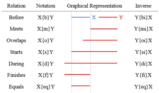
2.1 Allen’s Interval temporal relations . . . 7

2.2 (a) ITBN model for an activity in which X can happen before or during Y.

(b) BN representation of the ITBN shown in (a). . . 8

2.3 TR-LfD layered architecture. . . 11

2.4 Physical setup used during the data collection and validation user studies. . 12

2.5 Structure of the CNN models employed in the SRL. . . 14

2.6 Visualization of the window labeling process. . . 15

2.7 ITBN structure learned from the demonstrations of the behavioral intervention. 17

2.8 Example of perceptual aliasing. Each observation is mapped to a different

state by leveraging temporal reasoning. . . 18

2.9 Visualization of the policy selection process executed by the TRL. . . 20

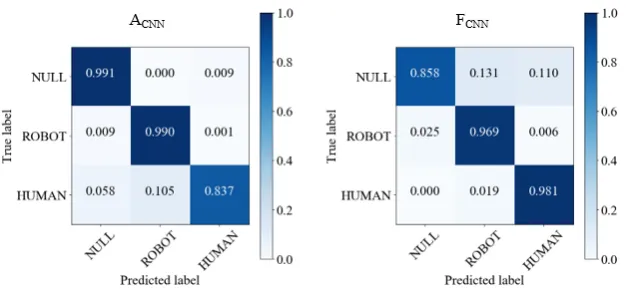
2.10 CNN performances on validation dataset. . . 22

3.1 Temporal relations captured by point-based (orange) and interval-based (green)

temporal reasoning models. . . 30

3.2 Physical setup used during the data collection user studies. . . 37

3.3 TCG models learned for the social greeting (a) and object naming (b) uses

cases. . . 38

C.1 Complete BN representation of the ITBN structure learned to model the social

(12)

LIST OF ALGORITHMS

1 Policy Selection in the TRL . . . 19

2 TCG Learning . . . 33

(13)

LIST OF ABBREVIATIONS

• ABA: Applied Behavior Analysis

• ASD: Autism Spectrum Disorder

• BN: Bayesian Network

• CNN: Convolutional Neural Network

• DAG: Directed Acyclic Graph

• DQN: Deep Q-Network

• DR-LfD: Deep Reinforcement Learning from Demonstration

• HRI: Human-Robot Interaction

• IA: Interval Algebra

• IRB: Institutional Review Board

• ITBN: Interval Temporal Bayesian Network

• ITR: Interval Temporal Relation

• LfD: Learning from Demonstration

• LSTM: Long Short Term Memory

• SD: Discriminative Stimuli

• SRL: Spatial Reasoning Layer

(14)

• TRL: Temporal Reasoning Layer

(15)

ABSTRACT

LEARNING TEMPORAL DYNAMICS OF

HUMAN-ROBOT INTERACTIONS FROM DEMONSTRATIONS

by

Estuardo Ren´e Carpio Mazariegos

University of New Hampshire, September, 2018

The presence of robots in society is becoming increasingly common, triggering the need to

learn reliable policies to automate human-robot interactions (HRI). Manually developing

policies for HRI is particularly challenging due to the complexity introduced by the human

component. The aim of this thesis is to explore the benefits of leveraging temporal reasoning

to learn policies for HRIs from demonstrations. This thesis proposes and evaluates two

distinct temporal reasoning approaches. The first one consists of a temporal-reasoning-based

learning from demonstration (TR-LfD) framework that employs a variant of an Interval

Temporal Bayesian Network to learn the temporal dynamics of an interaction. TR-LfD

exploits Allen’s interval algebra (IA) and Bayesian networks to effectively learn complex

temporal structures. The second approach consists of a novel temporal reasoning model, the

Temporal Context Graph (TCG). TCGs combine IA, n-grams models, and directed graphs

to model interactions with cyclical atomic actions and temporal structures with sequential

and parallel relationships. The proposed temporal reasoning models are evaluated using

(16)

indicate that leveraging temporal reasoning can improve policy generation and execution in

LfD frameworks. Specifically, these models can be used to limit the action space of a robot

during an interaction, thus simplifying policy selection and effectively addressing the issue

(17)

CHAPTER 1 INTRODUCTION

Robots are becoming more common in every day environments and activities, increasing

the need to learn robust policies for complex human-robot interactions. In this context,

a policy refers to the mapping between the states of the world and the actions that are

performed by a robotic system to accomplish a goal. Learning from Demonstration (LfD)

is a popular technique in robotics used to develop policies for the execution of a task from

a set of demonstrations [1]. LfD has been widely used to learn policies for low-level tasks

such as motion trajectories for obstacle avoidance [2], assembly operations [3–5], and tool

handling [6]. In contrast, little focus has been devoted to learning policies for high-level

tasks using LfD. Most of the existing approaches have concentrated on performing symbol

grounding and abstracting the goal configuration of a task [7–10].

Human-robot interactions are among the domains of high-level tasks that have barely

been explored by LfD research. Developing policies for these types of interactions is

chal-lenging due to the extensive variations that can exist in human responses to the same scenario

and the difficulties in detecting them reliably using multimodal perception techniques. The

work presented in [11] proposed an end to end deep reinforcement learning approach to learn

a simple human-robot greeting interaction from raw demonstration data. The approach used

a DQN to learn a reactive policy that performs policy selection based on features such as the

walking direction and head orientation of a passerby. In [12] a deep reinforcement learning

framework was employed to learn a behavioral intervention for children with autism

(18)

of temporal reasoning for policy selection. The results obtained in this work highlight the

importance of temporal reasoning in the process of learning policies for human-robot

interac-tions, specially to solve instances of perceptual aliasing. The problem of perceptual aliasing

occurs when a set of perceptual information can represent more than one of the states of

the task that is being observed. For example, in a human-robot interaction, a human may

exhibit the same response to two different stimuli but each response may lead to a different

action by the robot.

Temporal Reasoning has been integrated in LfD frameworks to simplify the perception

modules and address the issue of perceptual aliasing. Approaches that rely in finite state

machines and other simple graphical models [13, 14] can effectively learn simple temporal

structures but are not able to model tasks with repetitive atomic actions. More advanced

approaches based on Hidden Markov Models [15, 16] are able to model repetitive actions,

but can only learn sequential temporal relationships, namely before, after, equals.

The main objective of this thesis is to explore the benefits of leveraging temporal

reason-ing to learn policies for human-robot interactions from demonstrations. Particularly, how

temporal reasoning can be used to address the problem of perceptual aliasing, thus

simplify-ing the task of the perceptual modules. This thesis is divided into two main chapters. The

first highlights how leveraging temporal reasoningimpact positively impact the the reliability

of learned policies in a human-robot interaction context. The second chapter reports a novel

temporal reasoning model capable of addressing the limitations and weaknesses that have

been identified in other temporal reasoning approaches. A general overview of these two

chapters is included below.

Chapter 2 introduces a temporal-reasoning-based LfD (TR-LfD) framework to address

the challenge of developing policies for human-robot interactions. This framework was

de-signed to learn and leverage the temporal dynamics of a task. The TR-LfD employs an

architecture with three layers. First, a pre-processing layer prepares the perceptual data for

(19)

of classifying the preprocessed data to determine the state of the environment. Finally, a

temporal reasoning layer (TRL) performs policy selection based on the observations

pro-vided by the SRL and the temporal history of the interaction. The TRL relies on a temporal

reasoning model derived from an Interval Temporal Bayesian Network (ITBN) to learn the

underlying temporal structure of the task. This temporal reasoning model is capable of

encoding sequential and parallel relationships, however, its directed acyclic graph nature

prevents it from being able to model interactions with repetitive atomic actions.

Chapter 3 introduces a novel temporal reasoning model, the Temporal Context Graph

(TCG). This model encodes point-based temporal sequences using a directed graph and

combines Allen’s interval algebra [17] with n-gram [18] models to capture interval-based

relationships between the states represented by the nodes of the graph. Combining n-grams,

interval algebra and directed graphs allows TCGs to model tasks with repetitive atomic

actions, addressing the major shortcoming of the ITBN-based temporal reasoning model

employed in Chapter 2. TCGs also address the shortcomings of the approaches presented

in [15, 16] by employing interval algebra to encode the interval-based relationships that exist

between the atomic actions that take place in a task.

The TR-LfD and TCG approaches are evaluated in two IRB-approved studies to learn

policies for two different robot-mediated behavioral interventions from demonstrations. The

purpose of these interventions was to teach basic social/educational skills to children with

autism. The first intervention consists of an interaction between a child and his or her

therapist in which the latter teaches the former a greeting skill. The second use case consists

of an object-naming intervention where the therapist/teacher helps a child to improve his/her

vocabulary of everyday objects. Both interventions follow the principle of Appliled Behavior

Analysis. The performance of the frameworks is evaluated using quantitative and qualitative

methods. Results show that leveraging temporal reasoning can improve the performance

of policies generated with LfD approaches for human-robot interactions. Moreover, these

(20)

derivation could expedite the deployment of autonomous robotic platforms in scenarios where

(21)

CHAPTER 2 LEVERAGING TEMPORAL REASONING IN LEARNING

FROM DEMONSTRATION

2.1 Abstract

Understanding the rules that govern everyday interactions between humans and objects

requires identification and generalization of the key spatial and temporal features of the

interaction and modeling the high-level relationships between them. This chapter proposes

a novel Learning from Demonstration framework capable of learning complex interaction

dynamics. The framework relies on a Spatial Reasoning Layer to identify and generalize

spatial features and a Temporal Reasoning Layer to capture and analyze the high-level

temporal dynamics of an interaction. The proposed framework was first used to learn the

temporal structure and fundamental rules of a behavioral intervention and was then employed

to allow a robot to autonomously deliver that intervention to human participants, achieving

a successful performance in 84% of the sessions. The source code for this implementation is

available at https://github.com/AssistiveRoboticsUNH/TR-LfD.

2.2 Introduction

Learning from Demonstration (LfD) is a popular paradigm where the goal is to develop a

policy for performing a task based on a set of demonstrations provided by a human teacher

[1, 19]. LfD has been used to teach robotic systems low-level tasks such as generalizing

(22)

pick-and-place operations [20], or furniture assembly [3, 4]. However, learning high-level concepts

and abstract non-verbal reasoning from demonstrations is a field of LfD that has received

limited attention. The majority of research related to these topics has focused on abstracting

the spatial features of a task, disregarding its inherent temporal characteristics. Moreover,

these approaches use simplifying assumptions to identify the discriminatory features of the

different steps of a task. For example, the LfD frameworks in [7, 10] and [8] rely on

hand-picked features, simplifying assumptions and pre-defined conceptual spaces, respectively, to

perform symbol grounding and abstract the goal of pick-and-place operations.

In [11] an end-to-end deep reinforcement learning approach was used to learn a basic,

and unstructured social interaction from raw demonstration data. This model, however, was

designed to learn an interaction with low temporal dynamics in which policy selection could

be performed without performing temporal reasoning. In [21] a deep reinforcement learning

framework was designed to learn a high-level human-robot interaction. This framework,

although proficient in learning spatial reasoning, failed to learn the underlying temporal

rules that govern the interaction.

High-level activities such as human interactions with other humans or objects typically

have important underlying temporal structures that determine when low-level primitive

ac-tions are executed. Identifying these temporal structures, along with the spatial features, is

key to developing a holistic model of the activity. In this chapter a novel framework to learn

the dynamics of a structured social interaction from demonstrations is proposed.

Spatio-temporal reasoning is learned through a Spatio-temporal reasoning model which is designed based

on an Interval Temporal Bayesian Network (ITBN) [22]. ITBNs combine the well-developed

mathematical background of Bayesian Networks [23] with the temporal semantics of Interval

Algebra [17]. In the proposed LfD framework, spatial features of an interaction are learned

through a series of convolutional neural networks (CNN) [24] to enable the temporal

rea-soning model to learn and execute spatio-temporal inference. Results obtained from a user

(23)

of autonomous robots in human-robot interaction scenarios such as behavioral interventions

for children with autism spectrum disorder (ASD), a domain currently dominated by

tele-operated robots [25].

2.3 Background

2.3.1 Interval Algebra

Complex activities are composed of several events, each defined by a start and a stop time.

During the execution of an activity, events can happen simultaneously or in a sequential

manner, creating temporal relations and constraints between the events. Allen and Ferguson

[17] proposed a set of 13 atomic interval temporal relations that can exist between a pair of

events and limit the order in which events can take place in an activity (Fig. 2.1).

2.3.2 Interval Temporal Bayesian Networks

ITBNs are probabilistic graphical models designed to model the interval temporal relations

that exist between the individual events that constitute a complex activity [22]. This is

accomplished by combining Bayesian Networks (BN) with Interval Algebra. BNs are

graph-ical models capable of capturing conditional dependencies among random variables using a

directed acyclic graph (DAG). In an ITBN, each event of an activity is represented by a

(24)

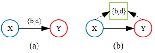
Figure 2.2: (a) ITBN model for an activity in which X can happen before or during Y. (b) BN representation of the ITBN shown in (a).

node in the DAG. Meanwhile, each edge of the graph represents the existence of a temporal

relationship between the two primitive events it connects. In an edge that goes from event

X to Y, X is the temporal reference of Y, meaning that Y has a temporal dependency on

X (Fig. 2.2).

Zhang et al. [22] proposed algorithms to perform structure and parameter learning on

ITBNs. They implemented ITBN as a BN by introducing a new set of nodes to represent

the temporal relationships between two event nodes (Fig 2.2). This approach allows ITBNs

to perform inference using existing BN algorithms. Therefore, the joint probability of the

nodes and links in an ITBN can be expressed as

P(Υ,Γ) =

n

Y

j

P(Yj|π(Yj)) K

Y

k

P(Ik|π(Ik)) (2.1)

where Υ and Γ represent the event nodes and temporal relation nodes, respectively. Yj is an

event node, Ik is a temporal relation node and π represents the parent nodes of the given

event or temporal relation.

Structure Learning

This process learns a graphical model that captures the spatio-temporal dynamics of an

(25)

all the events of an activity are learned using the concept of temporal distance:

d(ΩY,ΩX) = sY −sX, eY −eX, sY −eX, eY −sX

(2.2)

where X is the temporal reference of Y and Ω represents a tuple [s, e] containing the start

(s) and end (e) times of an event. The temporal distances for every possible pair of events

are then mapped to the atomic temporal relations listed in Fig. 2.1. Afterwards, an iterative

local search procedure [26] is used to generate new candidate networks. These structures are

evaluated using the Bayesian Information Criterion [27] to select the one that best fits the

training data.

Parameter Learning

This process involves finding a maximum likelihood estimate for the parameters of a model

from the training data. The algorithm is analogous to the parameter learning process of

BNs, with the exception that along with learning the conditional probability for each event

node, it is necessary to learn the conditional probability for the temporal relation nodes of

the model [22].

2.4 An LfD Framework for Learning Interaction Dynamics

The proposed LfD framework was trained to learn the dynamics of an applied behavior

analysis (ABA) style intervention from observations. ABA is a proven methodology used to

design behavioral intervention to teach social skills to children with ASD. The efficacy of the

selected ABA-style social greeting intervention was tested in a previous study [28]. During

this intervention a teacher and a child learner go through a series of structured interactions

with the purpose of teaching the child how to respond to a greeting in a socially acceptable

manner. The intervention begins with the teacher delivering a discriminative stimuli (SD)

(26)

respond (RESPONSE) verbally and/or wave his/her hand. If the child does not provide

an appropriate response, the teacher proceeds by delivering a prompt (PROMPT) which

directs the child how to respond in a socially acceptable manner, e.g. “John, say hi to me”.

If the intervention is failing to be productive, the teacher can decide to abort the session

(ABORT). If the child provides an appropriate response, the teacher concludes the session

by giving a verbal reward (REWARD) to the child, such as “Great job!”.

From an LfD perspective, learning the structure of such a high level interaction is

chal-lenging for different reasons. For example, the discriminative features can vary due to its

human component. Different teachers can deliver the intervention in different ways, using

different prompts, rewards and standards to define a session as a failure or success.

More-over, the reactions of different children to the same SD or prompts can vary greatly. The

interaction also follows a high-level temporal structure that needs to be learned in order to

accurately reproduce its dynamics. Using hand-picked features or hard-coding the

interven-tion, therefore, are inefficient, if not impossible.

The proposed LfD framework uses a layered architecture to learn and replicate the entire

interaction. A preprocessing layer refines the raw perceptual data, removing non-relevant

information. The preprocessed data is then used to train a set of CNN models in a spatial

reasoning layer (SRL) to identify discriminative features of different events in the

interven-tion. A trained SRL generates observations for the temporal reasoning model about the

state of the environment. The temporal reasoning model lies within the temporal reasoning

layer (TRL) and learns the spatio-temporal structure of the activity. The trained TRL can

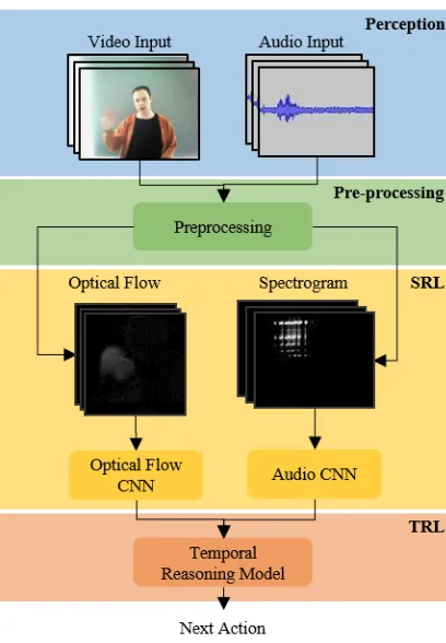
subsequently be used to replicate the demonstrated activity. Fig. 2.3 shows the structure

of the proposed framework. The different layers of the model are explained in the following

(27)

Figure 2.3: TR-LfD layered architecture.

2.4.1 Demonstration Data

An IRB-approved user study was organized in order to collect data to train the LfD

frame-work. In the user study, a NAO humanoid robot was tele-operated to deliver the ABA-based

intervention described above. The setup used during the data collection sessions can be

ob-served in Fig. 2.4. Since the robot was taking the role of the therapist, it was capable of

performing the following four actions: SD, PROMPT, REWARD and ABORT.

Six college students (4 male, 2 female) without ASD participated in the study. Before

starting the study, participants were made aware that the robot was being tele-operated.

Each participant completed a minimum of 18 interactions with the tele-operated robot. In

12 of the sessions the participants provided an appropriate response to the robot, thus ending

the session successfully and receiving a reward from the robot. The rest of the sessions ended

(28)

Figure 2.4: Physical setup used during the data collection and validation user studies.

consisted of different combinations of gaze, gestures, and audio, as defined below:

• Gaze: maintaining eye contact with the robot (Responses consisting of only gaze were not considered valid in this user study.)

• Gesture: responding to the robot with a waving gesture.

• Audio: acknowledging the robot with a verbal response, e.g. “hello”.

The dataset also included the temporal information (start and end times) of the events

that occurred in each intervention. The temporal data for the SD, PROMPT, REWARD

and ABORT actions was available from the tele-operation logs of each session. However, the

timing information for the participant’s responses were hand-labeled. The labeling process

consisted of analyzing the video and audio that preceded a REWARD action, to find the

start and end times of a response. The start of a gestural response was defined as the

first frame where the participant’s palm was visible. Similarly, the end frame was the last

one where the palm could be seen. Timing information for auditory responses was initially

obtained by processing the dataset with speech recognition software. However, these times

were identified manually in instances where the verbal response was not recognized by the

(29)

The collected dataset had a total of 189 demonstrations. All of the sessions included the

SD action, but only 133, 112, and 77 demonstrations included the PROMPT, REWARD

and ABORT actions, respectively. From the successful interactions, 74 contained gestural

responses and 75 had auditory responses. An evaluation dataset was created by randomly

selecting 25% of the demonstration videos.

2.4.2 Data Preprocessing Layer

The goal of the preprocessing layer is to refine and improve the quality of the information

received by the SRL. The video frames received from the robot are cropped to focus on

the human subject and their actions. Similarly, the audio feed is filtered to highlight the

participant’s response.

Video and audio data are recorded using the camera and microphones available on the

NAO robot. The image feed is recorded with the robot’s main camera, which provides

640 × 480 images at a rate of 15 frames per second. These images are cropped to be 299× 299 pixels in size and are centered on the participant’s face using a Haar Cascade classifier trained on human faces. Frames in which a face cannot be detected are cropped

using the center of the original image as a reference point. The resulting images are then

resized to 64×64 and converted to gray-scale. Finally, an optical flow image for each frame is generated using the change detection method described in [29]. The frames of the video

are then collected into an array F.

Audio data is preprocessed using a combination of spectral subtraction and finite

im-pulse response filters in order to reduce the audio signal’s background noise. The smoothed

data is subsequently converted to a Mel-Spectrogram in order to provide a two dimensional

representation of the data [30]. Finally, the resulting image is split into an array of frames

(A) equal in length to the number of frames in F. Each of the frames in A has dimensions

(30)

Figure 2.5: Structure of the CNN models employed in the SRL.

2.4.3 Spatial Reasoning Layer (SRL)

After the video and audio feeds are preprocessed, they are fed into the SRL. In this

imple-mentation, the SRL consists of independent CNN models forF andA. This approach allows

the framework to learn relevant audio and visual features without the potential of the model

over-fitting one of the input feeds. During training, the objective of the SRL is to extract

the discriminative features of each event in the demonstrated activity. During execution, the

SRL analyzes the preprocessed input to identify the current state of the environment and

provide observations to the TRL.

Long short-term memory (LSTM) cells were added to both CNN models to allow them to

learn low-level temporal features. LSTM layers can learn patterns from sequential data such

as frames in a video. These patterns can be used to identify complex features such as the

movement of a hand during a waving motion or specific auditory signatures. The detailed

structure of the SRL is shown in Fig. 2.5. The size of the filters (F), stride (S), number of

filters (N) and output size (O) is indicated for each layer

The CNN models process the input feeds using a sliding window approach, as shown in

Fig. 2.9. In this approach, the window size indicates the number of frames in a window,

and the frame stride is the number of frames skipped between adjacent windows. In this

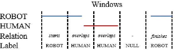
implementation, windows were classified as ROBOT, HUMAN, and NULL, as defined below:

(31)

Figure 2.6: Visualization of the window labeling process.

• HUMAN: frames that include gestural or auditory response provided by the human participant.

• NULL: frames that do not contain relevant information for either participant.

The label for each window was determined by using equation 2.2 to calculate the temporal

distance between the window and all of the events present in an intervention to identify the

interval temporal relations between them. A window was defined to belong to a class if

a during, overlaps, starts, f inishes or equals relation existed between an event and the

window (Fig. 2.6). The HUMAN class was given priority in this process when a window

could belong to more than one class.

Audio CNN

The input of the model for the auditory network (ACN N) is A, the visual representation of

the recorded audio. For the training process, a grid search approach was used to find the

window size and frame stride that maximized the number of windows that contain an entire

audio response from across the entire training dataset, without impacting the training time

of the CNN. As a result, the window size parameter was set to 20 frames and the frame

stride had a value of 7. For this model, the SD, PROMPT, REWARD, and ABORT actions

were grouped into the ROBOT class. The number of training examples of each class was

balanced by omitting excess windows belonging to the more common classes (ROBOT and

(32)

Optical Flow CNN

The optical flow CNN (FCN N) uses F as its input. During training, the window size and

frame stride parameters were set to 45 and 20 frames respectively. As in the case of ACN N,

the values of these parameters were selected using a grid search approach. The ROBOT class

captured the ambient movement caused by the waving motion of the robot when performing

the SD and PROMPT actions. The REWARD and ABORT actions were excluded from this

CNN as they did not include any motion from either of the participants in the intervention.

The same approach used in the training ofACN N for the balancing of training examples was

used for FCN N.

2.4.4 Temporal Reasoning Layer (TRL)

During training, the goal of the TRL is to learn and encode the underlying temporal dynamics

of the demonstrated interaction. During execution, this layer analyzes the observations

provided by the SRL to perform temporal reasoning and identify the event that is currently

taking place and, when necessary, decide which action should be executed next to complete

the current task.

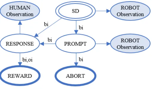
The TRL contains a temporal reasoning model developed using an ITBN as a reference.

This model is designed to perform policy selection and expand the capabilities of ITBNs

by modeling the waiting period between two events and using an open list to facilitate the

inference process. The temporal reasoning model (TRM) is defined as

T RM =G, Sn, Tn, St

(2.3)

where G is the graphical model of the activity, Sn is the set of start nodes of G, Tn is the

(33)

Figure 2.7: ITBN structure learned from the demonstrations of the behavioral intervention.

policy selection process and is defined as

St =

Oa, Ta, at−1, w

(2.4)

whereOa is an open list of events that can happen in the remainder of the interaction,Ta is

a list containing the times at which events have taken place, at−1 is the last event that was

observed in the interaction, and w is the time (in seconds) that the model will wait before

inferring the next action to execute.

The graphical structure and parameters of the temporal reasoning model are learned

from the temporal information in the training dataset. This information consists of a list of

events that occurred during an intervention, along with the event start and end times. As

a part of the structure learning phase, ROBOT observation nodes were attached for

non-terminal events related to the robot agent and a HUMAN observation node was attached

for events related with the human participant. The learned ITBN structure that models the

ABA intervention is shown in Fig. 2.7 (its BN equivalent can be found in Fig. C.1). In this

figure, the start node of the model is marked with a double line, terminal nodes are marked

with a thick line and observation nodes are shaded. The interval temporal relations in this

model can be read using the following structure: dependent node, followed by the temporal

(34)

Figure 2.8: Example of perceptual aliasing. Each observation is mapped to a different state by leveraging temporal reasoning.

can be read as “a response follows a prompt”.

During execution, the TRL is used to select the action that will be performed next in the

human-robot interaction. This policy selection process is governed by the temporal structure

of the task, which allows the TRL to address the problem of perceptual aliasing. This issue

arises when the perceptual information received by the model can be mapped to two different

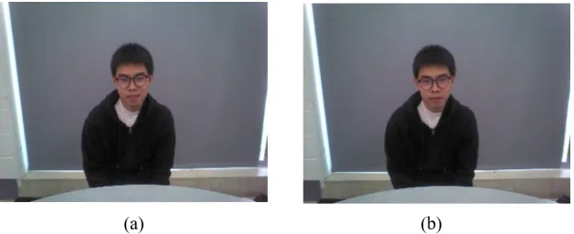
states of the task. An example of perceptual aliasing can be seen in 2.8, where both frames

display a non-compliant response from the participant. However, each one must be mapped

to a different state due to the temporal structure of the behavioral intervention. In this case,

frame (a) triggers a PROMPT action and, moments later, frame (b) triggers an ABORT

because a PROMPT had already been delivered during the intervention.

The algorithm used to perform policy selection in the TRL is shown in Algorithm 1.

This algorithm takes as input the set of observations generated by the SRL (obsSRL) and

the start (Ws) and end (We) times of the input window that generated those observations.

The value of the observation nodes for the TRL (obs) is decided based on obsSRL (line 4).

Any processed window can activate either the ROBOT observation nodes or the HUMAN

observation node. The ROBOT observation nodes are triggered when the ACN N classifies a

window as a ROBOT action. Meanwhile, the HUMAN observation node is triggered if either

the ACN N or the FCN N classify the window as a HUMAN action. ACN N is given priority

(35)

Algorithm 1Policy Selection in the TRL

Input: obsSRL, Ws, We

Output: at+1

1: initialize: Oa ← ∅,Ta← ∅, at−1 ← ∅ 2: if at−1 =∅ then

3: at+1 ←SD

4: else

5: obs← processObs(obsSRL)

6: if obs= NULL & w= 0 then

7: obs←ROBOT

8: end if

9: at+1, w ← inferNext(obs, Oa, Ta)

10: end if

11: if at−1 6=at+1 then

12: Oa= updateOpenList(at+1) 13: Ta ←Ta ∪(at+1, Ws, We)

14: at−1 ←at+1 15: else

16: updateEndTime(Ta, at−1, We)

17: w←w−1

18: end if return at+1

the REWARD and ABORT actions do not trigger the FCN N. To reduce the number of false

positives during execution, the model was configured to require two consecutive observations

to accept the detection of a HUMAN action.

The TRL uses the values ofobsalong withStfor policy selection (line 8). The event times

included inTa are used to calculate the interval temporal relations between past events and

an event that has been detected by the SRL. The temporal relation, along withOa, are then

used in the Bayesian inference process of the ITBN. This step is crucial in the process, as it

allows the TRL to perform temporal reasoning to resolve the issue of perceptual aliasing. For

example, if the SRL observes a ROBOT action and the SD is the only event that has occurred

in the session, the TRL will be capable of inferring that this new observation belongs to a

PROMPT action, because REWARD and ABORT events can only take place after a human

response or a PROMPT, respectively (Fig. 2.7).

(36)

Figure 2.9: Visualization of the policy selection process executed by the TRL.

response from the training dataset. This information is used during the inference process to

decide when to execute the next action in an automated intervention (line 5). The learned

values for these parameters were 7 and 3 seconds for the delay following a ROBOT action

and a HUMAN action, respectively. To select the next action, the TRL triggers the ROBOT

observation node (line 6) and then infers the appropriate action to execute based on the

current state of the intervention (line 10). The temporal reasoning model was implemented

using the Python package for graphical models, pgmpy [31].

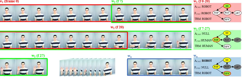
A brief example of the policy selection process is illustrated in Fig. 2.9. In this example,

the first window, w1 (red frame), consists of the last 20 frames of video corresponding to an

SD event. Both ACN N and FCN N classify w1 as a ROBOT action, triggering the ROBOT

observation nodes of the temporal reasoning model. In the graphical representation of the

TRL for w1, the current event is shaded with green, events that can still happen in the

intervention are white and the inferred event for the current window is marked with a red

line. After 7 more frames are received from the robot, a second window,w2 (green frame), is

processed. In this case, theFCN N classifies the window as a HUMAN action, so the HUMAN

observation node is triggered in the TRL. Using this observation, the TRL infers that the

window belongs to a RESPONSE action and updates the state of the model. Now, events

(37)

session are shaded with gray. Afterwards, a set of HUMAN action windows are received and

processed by the TRL, for simplicity these are not included in the figure. Finally, 3 seconds

after the response event ends, window wn (blue frame) is processed. In this window, the

TRL performs inference and selects REWARD as the next action to execute, thus ending

the interaction.

2.5 Results

2.5.1 Simulated Experiments

The learning capabilities of the framework were tested in simulation using the training and

evaluation datasets. During the simulated experiments, the preprocessing layer was used

to pre-process the demonstrations using a single window that covered all the frames of the

session. The window size and frame stride parameters of the CNN models were set to 20

and 7 frames, respectively.

The evaluation dataset was used to execute two different simulated experiments on the

framework. The first one, aimed to evaluate the individual performance of each CNN model

when used to classify the windows of the evaluation set. The results, which are shown on

Fig. 2.10, confirm that both models of the SRL were able to generalize and use the learned

features to classify novel windows with an accuracy of over 92%. Moreover, even though

the classification rate of ACN N for the HUMAN class was only of 83.72%, a more thorough

inspection revealed that all of the false negatives were late detections. This means that the

first HUMAN action window of an event was not classified correctly, but the subsequent

win-dows were. Therefore, during the delivery of an intervention, the event would be recognized

with a negligible delay or, in most cases, no delay at all.

In the second experiment, the TRL was used to infer which event was taking place

in each window given the observations provided by the SRL and the current state of the

temporal reasoning model. Since in this use-case the SD event is the only start node,

(38)

Figure 2.10: CNN performances on validation dataset.

framework was evaluated on the 139 training demonstrations, achieving a performance of

98.56% at the session level (two failed sessions). At the event level, the model achieved a

perfect performance for the SD, PROMPT, and ABORT events and a performance of 97.59%

on the RESPONSE and REWARD events. Then, the experiment was repeated using the

evaluation set, with a performance of 97.48% (2 of 50 sessions failed). Once again, the model

was able to achieve a performance of 100% on the SD, PROMPT, and ABORT events. The

two failed sessions were caused by false positives reported by the ACN N. From the results

of this experiment it is important to highlight that, even though the CNNs misclassified

a total of 184 windows on the first experiment described above, the TRL was able to use

its knowledge of the temporal dynamics of the interaction to reduce the number of failed

sessions to only two.

2.5.2 Experiments with Human Participants

To fully evaluate the learning capabilities of the framework, a new IRB-approved user study

was conducted. The setup and structure of the intervention were the same described in

section 2.4. In this study, however, the behavioral intervention was delivered autonomously

by the robot. Six college students (5 male, 1 female) without ASD participated in the study

and were made aware that the robot was acting autonomously. None of the participants

(39)

interactions that included different combinations of audio and gesture response, as well as

instances in which no response was provided.

There were two major differences in the operation of the framework in comparison to

how it had been employed in the simulated experiments. First, unlike in the simulated

experiments, the audio and video sequences were obtained in real time. Therefore, each

window needed to be preprocessed individually. As a consequence, the spectral subtraction

performed on the audio feed had to be executed using a noise sample from the training

dataset. The second fundamental difference was that, rather than recognizing the actions

that were being performed, the model was used for policy selection.

This experiment was executed using the policy selection routine described in Algorithm

1. An automated intervention started with the robot executing the SD action (line 4), as it

is the only start action in the TRL. Then the robot would act according to the participants

reaction. If no appropriate response was given, the robot would wait 7 seconds before

selecting the next action. If a valid response was received, the robot waited only 3 seconds

to generate the next action. The interventions continued until a terminal action (REWARD

or ABORT) was executed.

In this experiment, 84.26% of the automated interventions were successful (91 successful,

17 failures). An intervention was considered successful if the model allowed the robot to

react in accordance to the actions of the human participant and the state of the intervention

until the REWARD or ABORT actions were executed. A total of 11 failures were caused by

the misclassification of a ROBOT action by theACN N. Table 2.1 shows the performance of

the model at selecting the correct action after different combinations of human responses.

The accuracy in this table represents the percentage of responses that were followed by

the correct action by the robot. In addition, this table also includes the results obtained

by the Deep Reinforcement LfD (DR-LfD) approach described in [21] on the same ABA

intervention. A demonstration video of the performance of the system can be found at

(40)

Table 2.1: Accuracy of the TR-LfD framework on Automated Interventions

Responses

Gaze Gestural Auditory TR-LfD DR-LfD

No No No 94.4% 95.8%

No No Yes 100% 75.0%

No Yes No 91.7% 25.0%

No Yes Yes 83.3% 68.8%

Yes No No 94.4% 87.5%

Yes No Yes 91.7% 81.3%

Yes Yes No 100% 6.3%

Yes Yes Yes 100% 37.5%

Total 94.4% 67.8%

A questionnaire was completed by the participants of the evaluation user study. The

questions asked them to grade the performance of the automated robot and their overall

experience using a Likert scale with 5 meaning “strongly agree” and 1 “strongly disagree”.

The scores reflect that the robot learned to react correctly according to the actions of the

participants (4.5±0.5) and that, even though the automated intervention did not feel nat-ural (3.5±1.0), interacting with the robot was easy (4.8±0.4) and enjoyable (4.3±0.5). Nevertheless, the low score associated with the naturalness of the interaction is likely to be

a product of the highly structured nature of the intervention.

2.6 Discussion

The performance of the LfD framework on the evaluation set shows that the proposed

ap-proach is capable of learning complex activities from a reduced number of training

demon-strations. This is in part because the use of a TRL allows the simplification of the perception

models in the SRL. In this implementation, this was done by reducing the classes that needed

to be recognized by the SRL from 6 (SD, PROMPT, REWARD, ABORT, human response,

no response) to only 3 (ROBOT, HUMAN, NULL). Leaving the identification of the specific

robot or human action and, thus, the current state of the intervention to the TRL. As a

(41)

ROBOT, HUMAN and NULL classes from the small amount of training demonstrations

available (139 interventions).

The results also indicate the capacity of the framework to leverage the underlying

tem-poral dynamics of the activity to perform temtem-poral reasoning, even in cases when the SRL

provides incorrect observation values. This can be observed by comparing the results of the

two simulated experiments. In the first of these experiments, close to 5% of the windows

were misclassified. However, by using the learned rules and constraints of the interventions,

the TRL was capable of minimizing the effect of the misclassified windows, achieving a

per-formance of 98%. Lastly, it is relevant to point out that the proposed approach outperforms

the accuracy of the DR-LfD by 26.6%. This difference confirms the advantages of using

independent CNNs in combination with a temporal reasoning model when limited training

data is available.

The framework can be improved to increase its performance and make it more

general-izable to different use-cases. An approach to increase the performance would be to capture

noise samples in real time, before starting an intervention instead of using a prerecorded

sample. This is likely to decrease the misclassification rate of the ACN N.

2.7 Conclusion

This chapter presented a novel temporal-reasoning-based LfD framework that has been

proven capable of learning a complex human-robot interaction from demonstrations. The

framework relies on a SRL that extracts the discriminative features of the atomic events of

a demonstration and a TRL that derives and leverages the fundamental dynamics of the

activity. The framework was evaluated with a real use-case consisting of a human-robot

interaction. The results confirmed that the framework is capable of learning and replicating

complex activities, even when trained with a small number of demonstrations. This is made

possible by the integration of a temporal reasoning model that restricts the action-space and

(42)

the TR-LfD framework effectively deals with the problem of perceptual aliasing.

The results prove the feasibility of deploying LfD frameworks that leverage temporal

reasoning on applications that involve complex human-robot interactions. Future work could

explore the possibility of implementing video segmenting techniques to replace the

(43)

CHAPTER 3 TEMPORAL CONTEXT GRAPH

3.1 Abstract

High-level human activities are typically defined by rich temporal structures that determine

the order in which atomic actions are executed. To capture these temporal structures, this

chapter introduces the Temporal Context Graph (TCG), a temporal reasoning model that

integrates graphical and probabilistic models with Allen’s interval algebra. Bringing together

these three components, TCGs are capable of modeling tasks with cyclical atomic actions and

temporal structures with sequential and parallel relationships. Learning from Demonstration

is presented as the application domain where the use of TCGs can improve policy selection

and address the problem of perceptual aliasing. Experiments validating the model are

pre-sented for two tasks consisting of robot-mediated behavioral interventions. The source code

for this implementation is available at https://github.com/AssistiveRoboticsUNH/TCG.

3.2 Introduction

Learning from Demonstration (LfD) is a popular robot learning paradigm that learns task

policies from the demonstrations of a lay user [1]. In the context of LfD, a policy is the

mapping between the state of the world and the actions a robot can perform to complete a

task. LfD has been widely used in research to learn policies for low-level tasks such as motion

trajectories to perform obstacle avoidance [2], assembly tasks [4], and tool handling [6].

(44)

tasks such as object sorting [8], cooking related tasks [10,32], and the delivery of a behavioral

intervention [12]. Both in high and low-level LfD, tasks are composed of atomic actions that

need to be completed following a defined temporal structure to accomplish a goal. However,

several LfD approaches create policies by focusing on the spatial features of a task, failing

to take advantage of the implicit temporal structure that defines it.

This chapter introduces the Temporal Context Graph (TCG), a graphical model that

combines the temporal semantics of Allen’s interval algebra [17] with the probabilistic nature

of n-gram models to capture the temporal features of a task. TCGs can be used in LfD

frameworks to perform temporal reasoning and limit the action-space of the robotic agent,

simplifying the policy selection process. We validate the performance of TCGs in two

high-level LfD use cases in which the task is to learn a robot-mediated behavioral intervention.

3.2.1 Related Work

Different approaches have been explored in LfD literature to incorporate temporal features

in the policy creation process. The work reported in [33] employed a Hidden Markov Model

(HMM) approach to construct skill trees that implicitly encode the sequence in which atomic

actions are executed. Ekvall and Kragic [7] proposed learning a sequence of temporal

con-straints that could be used by a high-level planner during execution. A similar algorithm is

presented in [34], where tasks precedence graphs are introduced to encode spatio-temporal

constraints between atomic actions. Koenig and Mataric [32] proposed influence graphs to

model the sequence of events needed to complete a task. These simple graphical approaches,

however, are not capable of modeling tasks with repetitive atomic actions.

The approach described in [13] constructs finite state machines to model the temporal

relationships between atomic actions. Similarly, Manschitz et al. [14] proposed advanced

sequence graph learning algorithms to model tasks with repetitive actions. These models

use multi-class classifiers to learn and control state transitions, which allows them to learn

(45)

with perceptual aliasing. This occurs when a set of perception data can map to more than

one action, forcing the classifier to make an arbitrary selection.

The model described in [15] employs an extension of the Hierarchical Dirichlet Process

HMM (HDP-HMM) to address the problem of perceptual aliasing by learning a function

that can provide multi-valued mappings. Then, a set of perceptual data that triggers a

perceptual aliasing issue can map to multiple states, from which the HDP-HMM model

selects the most likely. In [16], the authors introduced the IBP (Indian Buffet Process) Coupled SPCM (Spectral Polytope Covariance Matrix)CRP (Chinese Restaurant Process)-HMM (ICSC-HMM), a Bayesian non-parametric model that prevents perceptual aliasing by identifying and learning sub-goals that encode key temporal dependencies in the task. These

models [15, 16], despite their robustness, can only recognize point-based temporal features,

meaning that they can only model three sequential temporal relationships, namely before,

after, and equals.

The Temporal Context Graph proposed in this chapter is a novel way of encoding the

temporal structures that are present in complex tasks. TCGs employ Allen’s interval

al-gebra to capture interval-temporal relations (ITR) among the atomic actions of the task.

These ITRs are then used to train n-gram models that prevent the TCG from failing due to

perceptual aliasing.

3.3 Preliminaries

3.3.1 Interval Algebra

Complex tasks can be decomposed into a set of atomic actions. Each of these actions

takes place over an interval of time that is defined by its start and end times. Allen and

Ferguson [17] identified a set of 13 atomic interval temporal relations (ITR) that can take

place between a pair of actions. These ITRs define and limit the order in which atomic

actions take place during a task and can be used to create a model of its temporal dynamics.

(46)

Figure 3.1: Temporal relations captured by point-based (orange) and interval-based (green) temporal reasoning models.

temporal models [15, 16] can only capture sequential ITRs (Fig. 3.1).

3.3.2 N-grams

N-grams [18] are a popular sequence modeling tool in the field of natural language processing.

N-gram models are utilized to simplify inference processes by using a set number of past states

to select the future one. The number of past states that are used in the inference process

is defined as N −1 where N is the order of the n-gram. These models have been used in speech recognition [35], text categorization [36], and sentence completion [37]. In a TCG

model, n-grams are used to perform policy selection based on the current temporal context

of the task, addressing the issue of perceptual aliasing.

3.4 Temporal Context Graph

3.4.1 Model Description

TCGs are temporal reasoning models capable of encoding the temporal structure of a task.

This is achieved by identifying the ITRs present between the atomic actions of the task and

using them to learn state transitions that depend on the temporal context of the task. The

temporal context of a task is composed by the set of actions and observations that have

(47)

Temporal Context Graphs are directed graphs for which each node represents a state

of the task and edges represent internal or external events that, combined with the current

temporal context, trigger a transition between two of these states. The TCG for a taskT at

a given timet can be formally defined as

T CGT ={N, E, P, St} (3.1)

where N is the set of states that can be reached during T, E is the set of edges connecting

the nodes in N, P is a set of probabilistic n-gram models used to model the transition

probabilities between two nodes of N, and S is the current state of the task, which is used

during execution to perform temporal reasoning.

Each nodeniin a TCG consists of a quintet{α, δ, ωn, τ, ϕ}whereαrepresents the atomic

action that should be executed whenni is reached,δindicates the duration ofα,ω indicates

the length of the waiting period between the completion ofαand the execution of a timeout

transition,τ indicates whether or not the node is a terminal state, and ϕindicates the order

of the n-gram model that needs to be used to perform temporal reasoning when the task

is transitioning from state ni. In a TCG, actions that generate a node are also referred to

as non-transition actions. Meanwhile, actions that give origin to an edge in the model are

called transition actions.

An edge ei in a TCG consists of a quartet {ηo, ηd, , ωe} where ηo and ηd represent the

origin and destination nodes, respectively, indicates the observed event or action that

triggers the transition, and ωe is the length of the waiting period between the completion of

and the execution of the atomic action indicated in nodeηd.

Transitions in TCGs are triggered by incoming observations of the state of the world and

are conditioned by the current temporal context of the task. State transitions in a TCG can

be of two different kinds,event transitions occur when an event or atomic action is observed.

(48)

is elapsed without observing any valid transition event. If an incoming observation cannot

trigger a transition given the current state and temporal context of the task, it is considered

aninvalid observation. These observations are treated as false positives and are disregarded

by the model when performing temporal reasoning.

3.4.2 Learning a TCG

Temporal Context Graphs are completely learned from a demonstration set and do not

require any parameter tuning or manual intervention. The three stages of the process are

outlined below and can be seen in Algorithm 2.

Demonstration Set

The input of a TCG model during the training phase is a set of demonstrations of a task.

Each of the individual demonstrations consists of a set of atomic actions. An action ai is

defined by a quartet {l, st, et,Γ} where l is a label used to identify the atomic action, st

and et are the start and end times, respectively, and Γ indicates whether or not ai should

be treated as a transition action. During the learning phase of a TCG it is assumed that

the training set provides the necessary information for all the atomic actions that define the

task.

Structure Learning

The first stage of the TCG learning process consists of learning the graphical structure for

the given task. The first step in this stage consists of sorting the atomic actions of the

training demonstrations, according to their start times (line 3). The atomic actions of each

sequence are then processed individually to learn the graphical structure that represents the

task. Nodes are created for each distinct non-transition action and transition actions are

used to create the edges connecting those nodes (lines 6-16). Additionally, timeout transition

(49)

The output of this algorithm can be considered a finite state machine that encodes the

point-based temporal relationships between the atomic actions of the given task. During

this process the mean duration and waiting periods for each atomic action are learned and

stored in the edges and nodes of the TCG (lines 17-22).

Algorithm 2TCG Learning

Input: D

Output: N, E, P

1: initialize: N ← ∅,E ← ∅, P ← ∅,IT R ← ∅

2: for d in D do

3: d←sort(d)

4: itr ← ∅

5: for actionin d do

6: next←action.next

7: itr←itr∪get itr(action, next, itr)

8: if ¬action.is transition then

9: if next.is transition then

10: next←next.next

11: transition←action.next

12: else

13: transition←T imeout

14: end if

15: E ←E∪edge(action, next, transition)

16: N ←N ∪action∪next

17: N.update duration(action)

18: if transition== T imeoutthen

19: N.update timeout(action, next)

20: else

21: E.update timeout(transition)

22: end if

23: end if

24: end for

25: IT R ←IT R∪itr

26: end for

27: orders←get required orders(IT R)

28: P ←learn ngrams(orders)

(50)

Table 3.1: ITRs in Terms of Temporal Distance

ITR sY −sX eY −eX sY −eX eY −sX

b <0 <0 <0 <0

bi >0 >0 >0 >0

d >0 <0 <0 >0

di <0 >0 <0 >0

o <0 <0 <0 >0

oi >0 >0 <0 >0

m <0 <0 <0 = 0

mi >0 >0 = 0 >0

s = 0 <0 <0 >0

si = 0 >0 <0 >0

f >0 = 0 <0 >0

fi <0 = 0 <0 >0

eq = 0 = 0 -

-ITR Sequence Generation

The second stage consists of generating a sequence of ITRs from the sequence of actions of

each demonstration. This is achieved by calculating the temporal distance between every

pair of consecutive atomic actions. The temporal distance for two actionsXandY is defined

as

d(ΩY,ΩX) = sY −sX, eY −eX, sY −eX, eY −sX

(3.2)

where X is the temporal reference of Y and Ω represents a tuple [s, e] containing the start

(s) and end (e) times of an atomic action. The results of this operation are used to identify

the ITR between the two actions using Table 3.1 [22].

During this stage ITRs that share a common temporal context are grouped and a group

identifier is added to the ITR sequence. This process, called ITR factoring, is necessary to

prevent the n-gram models to becoming too sparse.

Temporal Context Learning

The last stage starts by identifying the minimum order of an n-gram model that each node

(51)

set of ITRs obtained from the previous step are analyzed to identify the minimum number

of predecessors needed to eliminate the possibility of failing due to perceptual aliasing.

3.4.3 Policy Selection in a TCG

The policy selection process in a Temporal Context Graph consists of two steps that are

executed at each time step. The first is in charge of updating the state of the TCG with the

observations received from the environment. Meanwhile, the second step is used to verify if

a state transition needs to be triggered, prompting the TCG to select the next atomic action

to be executed. The state S of a TCG can be formally defined as

S ={n, o, s, t} (3.3)

where n is the current node of the TCG, o is the current observation of the environment, s

is the sequence that describes the current temporal context of the task, and tis the timeout

at which the next action will be selected and executed.

The state of the TCG is updated every time a new observation is received. At that

time, the model evaluates the possible transitions from the current node and discards the

observation if the transition is not valid. When a valid observation is received, the t and o

components of the state are updated and the new observation is added to s to update the

current temporal context of the task.

The actual policy selection process occurs when a timeout is reached. This routine, which

can be seen in Algorithm 3, starts by retrieving the n-gram model required by the current

node to perform policy selection. Then, the temporal context stored in s is used to retrieve

the sequence of ITRs needed by the n-gram model to complete the inference process. If a

valid atomic action is selected, the current node n, temporal context s, and timeout t are

updated to reflect the state of the task. When no valid action can be found, a defaultFailure

(52)

Algorithm 3Policy Selection in a TCG

Input: S, time

Output: action

1: initialize: action← ∅

2: if time > S.timeout then

3: n gram←P.get model(S.node.order)

4: itr ←generate sequence(S.context)

5: action←n gram.evaluate(itr)

6: if action==∅ then

7: action←F ailure

8: end if

9: S.node←action

10: S.sequence←S.sequence∪action

11: S.timeout ←(action.timeout+action.duration+time)

12: end if

13: return action

3.5 Evaluation Domain

The performance of the TCG was evaluated using two test cases of applied behavior analysis

(ABA) style interventions. ABA is a proven methodology used to design behavioral

inter-vention to teach social skills to children with ASD. Two IRB-approved user studies were

organized to collect demonstration data for the uses cases that are described in the

follow-ing sections. The physical setup utilized for both studies consisted of a NAO humanoid

robot that was being tele-operated to deliver the behavioral intervention. This setup can be

observed in Fig. 3.2.

3.5.1 Social Greeting Intervention

This intervention begins with a therapist delivering a discriminative stimuli (SD) by saying

“hello” and waving at a child. The child may respond (RESPONSE) verbally and/or wave

his/her hand. If the child does not provide an appropriate response, the teacher proceeds

by delivering a prompt (PROMPT) which directs the child how to respond in a socially

acceptable manner, e.g. “John, say hi to me”. If the intervention is failing to be productive,

(53)

Figure 3.2: Physical setup used during the data collection user studies.

response, the teacher concludes the session by giving a verbal reward (REWARD) to the

child, such as “Great job!”. Fig. 3.2 (a) shows an instance of this study in which the robot

is executing the SD action and waving at the participant.

A set of 139 demonstrations was used to train a TCG model for policy selection and a

pair of Convolutional Neural Networks (CNN) for perception. One of the CNNs was used

to classify the video feed from the camera on the NAO robot, the other classified the audio

feed coming from the robot’s microphone. In this use case the robot could perform four

actions: SD, PROMPT, REWARD and ABORT. In the TCG context, these four actions

were non-transition actions and were used to create the nodes of the graph. Meanwhile,

the only transition action was the RESPONSE provided by the human participant. The

structure of the TCG learned for this use case is shown in Fig. 3.3 (a).

3.5.2 Object Naming Intervention

In this behavioral intervention a therapist delivers a discriminative stimuli (SD) to a child

by asking them to name an object that is present on the table and pointing at it. The

child may provide a CORRECT or INCORRECT verbal response. If the child does not

provide an appropriate response, the teacher proceeds by delivering a prompt (PROMPT)

(54)

Figure 3.3: TCG models learned for the social greeting (a) and object naming (b) uses cases.

basketball. Can you tell me what this is?”. If the intervention not being successful, the

teacher can provide more prompts (PROMPT) or decide to abort the session (ABORT).

If the child provides an appropriate response, the teacher concludes the session by giving

a verbal reward (REWARD) to the child, such as “Great job!”. Fig 3.2 (b) displays the

physical setup used for this user study.

In this intervention the robot could perform the same four actions as in the social greeting

intervention, with the peculiarity that the PROMPT action could be delivered repeatedly.

The TCG learned for this intervention is shown in Fig 3.3 (b). This model was learned from

a set of 127 demonstrations. This use case employed only one CNN for perception, as the

video feed contained no relevant information for the interaction.

3.5.3 Experimental Results

The first use case highlights the importance of performing temporal reasoning during policy

selection. This is because of the perceptual aliasing issue that exists between the observations

that trigger a PROMPT and ABORT action on the robot. The policy selection capabilities