ISSN: 2278-067X, Volume 1, Issue 3 (June 2012), PP.37-44
www.ijerd.com
Development of Mathematical Models for Various PQ Signals
and Its Validation for Power Quality Analysis
Likhitha.R
1, A.Manjunath
2, E.Prathibha
3Department of EEE Sri Krishna Institute of Technology, Bangalore, Karnataka
Abstract— PQ analysis for detecting power line disturbances in real-time is one of the major challenging techniques that are being explored by many researchers. In order to understand the causes of electronic equipment being damaged due to disturbances in power line, there is a need for a robust and reliable algorithm that can work online for PQ analysis. PQ signal analysis carried out using transformation techniques have its own advantages and limitations, In this work, Mathematical models for various PQ signal disturbances is developed and validated against real time signal. Based on the mathematical models developed, performances of various transformation techniques are compared. Software reference models for transformation techniques are developed using MATLAB. The developed models are verified using various signal disturbances.
Keywords— Power quality, Power system transients, discrete wavelet transforms. Lifting based wavelet transform.
I.
INTRODUCTION
In recent years power quality has became a significant issue for both utilities and customers. This power quality issue is primarily due to increase in use of solid state switching devices, non linear and power electronically switched loads, unbalanced power system, lighting controls, computer and data processing equipments as well as industrial plants rectifiers and inverters. PQ events such as sag, swell, transients, harmonics and flicker are the most common types of disturbances that occur in a power line. Sophisticated equipment’s connected to the power line are prone to these disturbances and are affected or get damaged due to disturbances that randomly occur for very short durations. Thus, it is required to estimate the presence of disturbance, and accurately classify the disturbances and also characterize the disturbances. In order to perform the tasks such as detection, classification and characterization, it is required to understand the basic properties of PQ events and their properties. In this section, PQ events (like sag, swell, transients, harmonics and flicker) and their properties are summarized.
II.
REPRESENTATION OF PQ SIGNALS AND THEIR PROPERTIES
PQ signals such as sag, swell, transients, harmonics and flicker have some very basic properties in terms of signal amplitude and frequency as governed by standards ie 220 V and 50Hz signal. Variations in voltage levels and variations in frequencies lead to disturbances in PQ signal. Frequency variations in PQ signals introduce harmonics, random change in loads lead to transients, flicker, sag and swell. Figure.1 shows the different types of disturbances that occur in PQ signal.
From Figure 1 we define the disturbances as follows [1-4]:
Voltage variation: increase or reduction in the amplitude of the voltage normally caused by variations in the load. Voltage variation can be termed as swell or sag.
Voltage sag: sudden reduction in the rms voltage to a value between 0.9 pu and 1pu of the declared value (usually the nominal value) and duration between 10 ms and 1 min.
Voltage swells: sudden increase in the voltage to a value between 1.1 pu to 1.8 pu and duration between 10 ms to 1 min Transient: oscillatory or non-oscillatory over voltage with a maximum duration of several milliseconds.
Flicker: intensity of the nuisance caused by the flicker, measured as defined by UIE-CEI and evaluated as: -Short term flicker (Pst) measured in 10 minutes period
-Long term flicker (Plt) defined as 3
12
1 3
12
ist lt
P
P
Figure.1 graphical representations of PQ signal disturbances
III.
MATHEMATICAL MODELING OF PQ SIGNALS
Verification of software reference models for PQ analysis requires PQ signals; which are generated using software programs. In order to represent the real time signals accurately, mathematical equations are used to generate PQ Synthetic signals. Synthetic signals generated need to have all the properties of a real-time signal and should match the real-time signal in all aspects. Performance of PQ analysis techniques is dependent of PQ signals, hence it is required that the synthetic signals which are generated using software programs are accurately modeled. Development of software programs to generate PQ signal disturbances are governed by standard definitions [5-7] for events as given in Table 1 is generated.
Table1. Mathematical Models of PQ Signals
PQ disturbances Model Parameters Normal x(t)=sin(ωt)
swell x(t)=A(1+α(u(t-t1
)-u(t-t2)))sin(ωt)
t1<t2,u(t)= 1,t≥0
0,t<0
0.1≤α≤0.8 T≤t2-t1≤9T
Sag x(t)=A(1-α(u(t-t1
)-u(t-t2)))sin(ωt)
0.1≤α≤0.9;T≤t2-t1≤9T
Harmonic x(t)=A(α1sin(ωt)+α3
sin(3ωt)+ α5
sin(5ωt)+ α7sin(7ωt))
0.05≤α3≤0.15,
0.05≤α5≤0.15 0.05≤α7≤0.15,∑αi
2
=1
Outage x(t)=A(1-α(u(t-t1
)-u(t-t2)))sin(ωt)
0.9≤α≤1;T≤t2-t1≤9T
Sag with
harmonic
x(t)=A(1-α(u(t-t1
)-u(t-t2)))
(α1sin(ωt)+α3sin(3ωt
)+ α5 sin(5ωt))
0.1≤α≤0.9,T≤t2-t1≤9T
0.05≤α3≤0.15,
0.05≤α5≤0.15; ∑αi2=1
Swell with harmonic
x(t)=A(1+α(u(t-t1
)-u(t-t2)))
(α1sin(ωt)+α3sin(3ωt
)+ α5 sin(5ωt))
0.1≤α≤0.9,T≤t2-t1≤9T
0.05≤α3≤0.15,
0.05≤α5≤0.15; ∑αi2=1
Interruption x(t)=A(1-(u(t2
)-u(t1)))cos(𝜔t)
Transient x(t)=A[ cos(𝜔t)+k cxp(-(t-t1)/τ)
cos(ωn(t-t1))(u(t2
)-u(t1))]
K=0.7 τ=0.0015 ωn=2 𝜋fn
900≤fn≤1300
x(t)- PQ signal, A-Amplitude(constant), n-angular frequency, t-time,
n-time duration of event occurrence (constant), T-time duration, fn
-frequency, K-constant, τ-constant
Sag and swell events are modeled using step functions defined for periods between t1 and t2, amplitude of step
function is used to control the intensity of voltages thus defining sag and swell. Time intervals t1 and t2 define the
duration of sag and swell. Harmonic signal consists of frequency components that are multiples of 1 KHz. In a PQ signal the disturbances in terms of harmonics will have more than three frequency components and are odd multiples of fundamental component. The odd harmonics also have voltage Variations and thus affect the fundamental signal. Parameters that define amplitudes of harmonic components given by α1, α2, α3 and α4 have variations from 0.05 to 0.15
and the square sum of all components should not exceed unit magnitude. These parameters are used to control the harmonic variation in a pure sine wave signal.
In signal disturbances that create exponential variations within a short duration of time interval are transients. Parameters such as α, w and K control the variations in transients in a given pure sine wave as shown in table 1. Transients occur for a short time interval, controlled by t1 and t2. During this time interval, the signal behaviors consists
an exponential variation controlled by τ. Flicker is due to randomness in sag and swell affecting pure sine wave. Mathematical models for flicker are similar to sag and swell, but the duration of sag and swell is randomly added to the pure sine wave signal.
IV.
ALGORITHM FOR PQ SIGNAL GENERATION USING MATHEMATICAL
MODELS
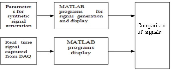
Based on the discussions and numerical equations presented in the previous section software programs are developed for modeling PQ signals with disturbances as shown in Figure 2. Control parameters for variations in distortions or events are defined as user inputs. The known disturbances are introduced in the signal; graphical display helps in verifying the PQ events.
Figure 2: Block diagram for signal generation using mathematical models
V.
FLOW CHART FOR PQ SIGNAL DISTURBANCE GENERATION USING
MATLAB
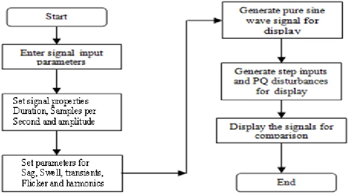
Figure 3 presents the flow chart for the PQ signal disturbances generation using MATLAB. PQ signal of 50 Hz for duration of 10 seconds with sampling rate of 1 ksps consisting of 400,000 samples are generated. Generated signals are divided into frames of 1024 samples. The MATLAB program is simulated with the required parameters depending upon user requirements. The disturbances are introduced and generated signals are displayed for visualizations.
VI.
SIMULATION RESULTS OF PQ SIGNALS USING SOFTWARE PROGRAMS
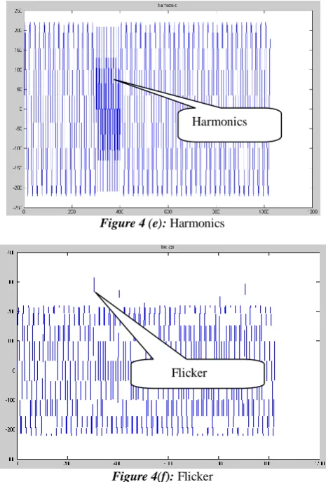
Software programs discussed in previous section is simulated using MATLAB, the results of the same is presented in this section. Pure sine wave, sag, swell, transients, harmonics and flickers signals are generated and displayed as shown in Figure 4(a-f). PQ signal with 50 Hz, 220 V peak is sampled at 1 Ksps, is introduced with disturbances and is plotted.
Figure4 (a): sine wave
Figure4 (b): Voltage swell
Figure 4 (c): Voltage sag
Figure 4 (d): Voltage transients
Voltage transients Voltage swells
Figure 4 (e): Harmonics
Figure 4(f): Flicker
Disturbances in PQ signal with variations in various parameters like amplitude and duration are generated and recorded for the analysis. Database of more than 120 signals are generated and are used for classification and characterization. Table 2 presents various test cases that have been generated using the software models and the generated signal is compared with real time signals.
VII.
REAL TIME GENERATION OF PQ EVENTS:
In order to validate the mathematical models that are used to generate PQ disturbances, it is required to verify the correctness of synthetically generated signal against real time signals. Hence it is required to generate and capture real time disturbances. Figure 5 shows the block diagram for the experimental set-up to acquire real time PQ disturbances for the analysis. Experimental set up consists of a power line connected to data acquisition system, loads such as resistive (lighting load or lamp), inductive load (induction motors) and both. Voltage variation across the power line is captured using the data acquisition system consisting of differential module, ADC to digitize the analog signals to 12-bit resolution and software for data acquisition and data processing. The DAQ (Data Acquisition) card (PCL818HG) [62] and driver software SNAP MASTER is used for data capture and AUTO SIGNAL ANALYSIS software for analysis.. The line voltage is captured from the distribution node, and conditioned to step down the voltage to ± 10V. The stepped down voltage is converted to its digital equivalent using the DAQ card, the digital data is further processed using software modules. The processed data is displayed for visualization and information is extracted for analysis.
Power supply 230V
Differential
Module A/D card
CPU Computer
Monitor
Figure 5: Block diagram for the experimental set-up
A GUI is developed to automate the experimental setup. This helps in selecting the instruments required for measurement. Types of ADCs, properties of ADCs, signal interfaces and display mode settings can be configured using
Harmonics
the GUI [63]. GUI also helps in defining sampling rate, duration of frame length, and number of frames that needs to be captured for data processing. The start duration and stop duration that can be set in the GUI helps in capturing the PQ signal at the required time for processing. Data captured using the data acquisition unit stores the captured data in ASCII format and *.plt format is used for analysis. Loads are varied to introduce PQ disturbances and the captured data is taken for analysis. Variations in load such as resistive and inductive are randomly introduced and multiple experiments are conducted.
VIII.
VALIDATION OF MATHEMATICAL MODELS
In order to check the correctness of the developed mathematical models and it is required to validate the generated synthetic signal against real-time signals. In this work, an experimental setup is developed to generate real-time signal and disturbances are introduced by varying different loads. The data acquisition unit developed captures the signal along with the disturbances. The recorded signal is stored in a text file. The MATLAB model developed reads the text file and the contents are plotted. The software program developed based on mathematical model is used to generate similar kind (real-time) of signal by varying the input parameters to the software model. The output of both the software model and the real-time signal are compared and modifying the mathematical models minimizes the error between them. Various test cases are captured using the real-time experimental setup, which are used to verify the synthetic signal generated using software programs. The synthetic signal is validated against real-time signal and is used for PQ analysis. Figure 6 shows the experimental set up for PQ signal validation.
Figure 6: Experimental setup for PQ signal validation
Comparison or equivalence check is carried out to compare the similarities between real time PQ signal and synthetic PQ signal. Synthetically generated PQ signal is compared with the results of real time signals. In order to compare the signals Mean Square Error (MSE) [64] is computed between the real time signal and the synthetic signal as in equation
𝑴𝑺𝑬 =𝟏
𝑸 𝒆(𝒌)
𝟐 𝑸
𝒌=𝟏
=𝟏
𝑸 (𝒕 𝒌 − 𝒂 𝒌 )
𝟐 𝑸
𝒌=𝟏
t(k) is the real time signal samples that are compared with a(k) which is the generated synthetic signal, Q is number of samples. The difference in samples values are squared and accumulated to compute MSE. Real time signals generated for various disturbances is compared with synthetic signal, the MSE is verified, MSE is well above threshold value of 2%, mathematical model presented in Table1 is modified to minimize the MSE well below the threshold.
IX.
SUMMARY OF VALIDATIONS
Table 2 Real time signal validation results
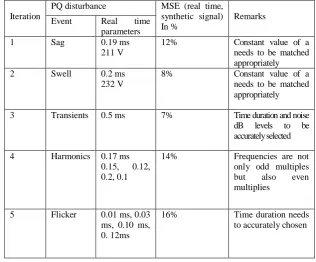
From the results obtained it is observed that MSE is greater than the required threshold level which is 2 %, this variations is due to the fact that the mathematical models that have been tabulated in Table 3 does not accurately model the real time signals. In order to minimize the error, it is required to appropriately update the mathematical model for PQ signal generation. The major limitation is that the real time signal parameters obtained have to be appropriately introduced in to the mathematical model i.e need to choose appropriate time interval, intensity values for events and select appropriate harmonics levels. The modified mathematical models that match with the real time signals are presented in Table 3
Table 3 Modified mathematical models Iteration
PQ disturbance MSE (real time, synthetic signal) In %
Remarks Event Real time
parameters
1 Sag 0.19 ms
211 V
12% Constant value of a needs to be matched appropriately
2 Swell 0.2 ms
232 V
8% Constant value of a needs to be matched appropriately
3 Transients 0.5 ms 7% Time duration and noise dB levels to be accurately selected
4 Harmonics 0.17 ms 0.15, 0.12, 0.2, 0.1
14% Frequencies are not only odd multiples but also even multiplies
5 Flicker 0.01 ms, 0.03 ms, 0.10 ms, 0. 12ms
16% Time duration needs to accurately chosen
PQ disturbanc es
Model Parameters and mathematical models
Modified mathematical models and parameters
Normal x(t)=sin(ωt) x(t)=sin(ωt)
Swell
x(t)=A(1+α(u(t-t1
)-u(t-t2)))sin(ωt)
0.1≤α≤0.8 T≤t2-t1≤9T
x(t)=A(1+α(u(t-n*t1
)-u(t-m*t2)))sin(ωt)
0.1≤α≤0.8 T≤t2-t1≤9T
Sag x(t)=A(1-α(u(t-t1
)-u(t-t2)))sin(ωt)
0.1≤α≤0.9;T≤t2-t1≤9T
x(t)=A(1-α(0.2*u(t-n*t1
)-u(t-m*t2)))sin(ωt)
0.1≤α≤0.9;T≤t2-t1≤9T
Harmonic x(t)=A(α1sin(ωt)+α3si
n(3ωt)+ α5 sin(5ωt)+
α7sin(7ωt))
0.05≤α3≤0.15,0.05≤α5
≤0.15
0.05≤α7≤0.15,∑αi2=1
x(t)=A(α1sin(ωt)+α3sin(3ωt)
+α5 sin(5ωt)+ α7sin(7ωt)
+α4sin(4ωt))
0.05≤α3≤0.17,0.05≤α5≤0.25,
0.05≤α4≤0.12
0.05≤α7≤0.35,∑αi2=1
Transient x(t)=A[cos(𝜔t)+k cxp(-(t-t1)/τ)
cos(ωn(t-t1))(u(t2
)-u(t1))]
K=0.7τ=0.0015 ωn=2 𝜋fn
900≤fn≤1300
x(t)=A[ cos(𝜔t)+k cxp(-(t-t1)/τ)
cos(ωn(t-n*t1))(u(m*t2
)-u(n*t1))]
K=0.7τ=0.0015 ωn=2 𝜋fn
900≤fn≤1300
x(t)- PQ signal, A-Amplitude(constant), n-angular frequency,
t-time, n-time duration of event occurrence (constant), T-time
The modifications are that the time periods of event disturbances are accurately controlled by n and m constants. The intensities of events are also modified by appropriately choosing the constants. The modified equations are modeled using MATLAB software constructs and the results generated are compared with real time signals after several iterations, the MSE was brought below 2% threshold. Thus the mathematical models that have been modified are matching the real time PQ event disturbances and thus are used for analysis.
X.
CONCLUSION
In this paper mathematical model for PQ signal generation is developed and is validated against real time PQ signal. PQ events such as sag, swell, transient, and harmonics are generated using the mathematical model developed. Real time signals generated consisting PQ disturbances are compared with the results of synthetic signals.. MSE is computed between the synthetic and real time signal. Voltage sags and swells intensities and duration of occurrence is noted from real time results, the same parameters are set in the synthetic model. From the results obtained it is observed that MSE is greater than the required threshold level which is 2 %, In order to minimize the error, it is required to appropriately update the mathematical model for PQ signal generation.
REFERENCES
[1]. IEEE Task Force (1996) on Harmonics Modeling and Simulation: Modeling and Simulation of the Propagation of Harmonics in Electric Power Networks – Part I: Concepts, Models and Simulation Techniques, IEEE Trans. on Power Delivery, Vol. 11, No. 1, pp. 452-465Santoso .S., Grady W.M., Powers E.J., Lamoree J., Bhatt S.C., Characterization of Distribution power quality events with Fourier and wavelet transforms. IEEE Transaction on Power Delivery 2000;15:247–54.
[2]. Probabilistic Aspects Task Force of Harmonics Working Group (Y. Baghzouz Chair) (2002): Time-Varying Harmonics: Part II Harmonic Summation and Propagation – IEEE Trans. on Power Delivery, No. 1, pp. 279-285Meyer.Y., Wavelets and Operators. Cambridge University Press, 1992,LondonUK.
[3]. R. E. Morrison,(1984) “Probabilistic Representation of Harmonic Currents in AC Traction Systems”, IEE Proceedings, Vol. 131, Part B, No. 5, pp. 181-189Pillay, P., Bhattacharjee, A., Application of wavelets to model short-term Power system disturbances. IEEE Transactions on Power Systems ,1996. 11 (4), 2031– 2037.
[4]. P.F. Ribeiro (2003) “A novel way for dealing with time-varying harmonic distortions: the concept of evolutionary spectra” Power Engineering Society General Meeting, IEEE, Volume: 2 , 13-17, Vol. 2, pp. 1153Karimi, M., Mokhtari, H., Iravani, M.R., Wavelet based on line disturbancedetection for power quality applications. IEEE Transactions on Power Delivery, 2000. 5 (4), 1212–1220.
[5]. Haibo He and Janusz A (2006) “ A Self-Organizing Learning Array System for power quality classification based on Wavelet Transform” IEEE Trans.Power Delivery, vol. 21, no.1, pp. 286-295. C.Sharmeela ,M.R.Mohan,G.Uma and J.Baskaran., A Novel Detection and classification Algorithm for Power Quality Disturbances using wavelets.American journal of applied science 2006 3(10):2049-2053
[6]. T.K.A. Galil, M. Kamel.A.M. Yousssef, E.F.E. Saadany, and M.M.A. Salama (2004). “Power quality disturbance classification using the inductive inference approach”, IEEE Trans.Power Delivery, vol. 19, no.10, pp. 1812-1818.
[7]. J.Starzyk and T.H.Liu,(2003) “ Self-Organizing Learning Array”IEEE Transaction on Neural Netw..vol.16 no.2,pp.355-363.