A Modified Particle Swarm Optimization Algorithm for Reliability Redundancy Optimization Problem

(1)

A Modified Particle Swarm Optimization

Algorithm for Reliability Redundancy

Optimization Problem

Yubao Liu

College of Computer Science and Technology, Jilin University, Changchun, China College of Computer Science and Technology, Changchun University, Changchun, China

Email: [email protected], [email protected]

Guihe Qin*

College of Computer Science and Technology, Jilin University, Changchun, China

Key Laboratory of Symbolic Computation and Knowledge Engineering of Ministry of Education, Jilin University, Changchun, China

Email: [email protected]

Abstract—In this paper, a modified particle swarm optimization (MPSO) algorithm is proposed to solve the reliability redundancy optimization problem. This algorithm modifies the strategy of generating new position of particles. For each generation solution, the flight velocity of particles is removed. Whereas the new position of each particle is generated by using difference strategy. Moreover, an adaptive parameter is used to ensure diversity of feasible solutions. Experimental results on four benchmark problems demonstrate that the proposed MPSO has better robustness, effectiveness and efficiency than other algorithms reported in literatures for solving the reliability redundancy optimization problem.

Index Terms—nonlinear programming, PSO, reliability optimization, redundancy allocation, adaptive mechanism

I. INTRODUCTION

The reliability optimization problem is very important in industry and has attracted attention in academic field and engineering fields. In general, two major ways have been used to improve system reliability. The first way is by increasing the reliability of components, and the second way is by using redundant components in the subsystems. In the first way, sometimes it cannot meet our requirements even though the currently highest reliable components are used. The second way is by choosing the components reliability combination and redundancy levels to arrive the highest system reliability. Whereas the cost, weight, volume will be increased as well. So it is necessary that a trade-off is achieved between these two options for constrained reliability optimization. Such reliability allocation and redundancy

allocation problem is called as RRAP (reliability redundancy allocation problem) [1, 2 , 3].

RRAP has been proven to be NP-hard problem [2]. So far many different optimization technologies have been presented to resolve it. Exact optimization methods provide exact optimal solution and have been found to be suitable for small-size problems. But real world problems may have large sizes and involve many constraints. And even multiple components are chosen for each subsystem to enhance reliability. Because of the computational difficulty that increases exponentially in terms of problem size, the approaches called heuristics and meta-heuristics have been widely researched and applied[6,10].They offer feasible solution within reasonable computational time.

There are four reliability-redundancy allocation problems of maximizing the system reliability subject to multiple nonlinear constraints[7,12]. They are nonlinearly mixed-integer programming problems and are formulated as following model uniformly [4, 39 , 41]:

Max Rs = f(r,n)

s.t.

gj(r,n)≤bj,j=1,…,m, nj∈positive integer, 0≤rj≤1 (1)

Where ri is the reliability of subsystem i, and ni is the

number of components of subsystem i. The f(.) is the objective function for the system reliability; the gj(.) is

the jth constraint function and bj is the jth upper

limitation of the system; the m is the number of subsystems. The goal is to determine the number of redundant components and the components’ reliability in each subsystem so as to maximize the overall system reliability. This problem belongs to the category of constrained nonlinear mixed-integer optimization problems.

For solving the system reliability optimization problems, many researchers had paid great effort and presented many efficient methods. Prasad and Kuo presented implicit enumeration [9], and F.S. Hiller etc.

Manuscript received September 16, 2013; revised February 16, 2014; accepted March, 2014.

(2)

presented dynamic programming [5] and branch-and-bound [11] to solve the reliability-redundancy allocation problem. But they are high time-consuming when the problem size is larger. With the development of artificial intelligence, some meta-heuristics methods have been proposed. Hsieh [8] used a linear programming approach to solve the RRP-MCC with nonlinear constraints. Coit and Smith[18] presented a genetic algorithm (GA) to solve the Reliability-Redundancy problem. Hsieh et al. [14] used genetic algorithm to solve reliability design problems of series systems, series-parallel systems and complex (bridge) systems. You and Chen [15] proposed a greedy genetic algorithm for series–parallel redundant reliability problems. Ta_Cheng Chen [16] used an immune algorithm-based approach to solve the RRP-MCC problem of series system, series–parallel system, and complex (bridge) systems and overspeed protection system. Hsieh and You [17] presented an immune based two-phase approach to solve the reliability-redundancy allocation problem. First, an immune algorithm (IA) is used to get preliminary solutions. Second, the quality of solutions was improved by a procedure to obtain the last solutions. The result showed that the solutions are superior to those best solutions of other approaches in the literature. Liang and Chen[13] proposed a variable neighborhood search (VNS) with an adaptive penalty function. This method improved the performance and the solution quality were as good as others. Zavala et al.[21] proposed a particle swarm optimization (PSO) approach named PESDRO to solve a bi-objective redundant reliability problem; And the reliability redundant problems of series system, parallel system and K-out-of-N system are resolved. Zou et al. [19, 20] used global harmony search algorithm to solve RRAP. Leandro dos Santos Coelho [22] presents a PSO approach based on Gaussian distribution and chaotic sequence (PSO-GC) to solve the reliability–redundancy allocation problems of complex (bridge) system and overspeed protection system. The PSO-GC has got better solutions than the classical PSO. Harish Garg and S.P. Sharma [38] used PSO to solve multi-objective reliability redundancy allocation problem of a series system. Agarwal and Sharma[26] applied ant colony optimization(ACO) algorithm with an adaptive penalty function to redundancy allocation problem. Nabil Nahas et al. [25] coupled ant colony optimization algorithm with degraded ceiling local search method for redundancy allocation of series–parallel systems. Mohamed Ouzineb[24] presented tabu search(TS) approach to solve the redundancy allocation problem for multi-state series–parallel systems. Afonso et al.[29] used imperialist competitive algorithm

(ICA) to resolve RRAP. Recently some hybrid meta-heuristic methods have

been proposed to solve the reliability redundant allocation problems. Nima Safaei et al.[28] presented an Annealing-based PSO (APSO) method. Even though APSO didn’t obtain the better solution than other well-known meta-heuristic method, it applied Metropolis-Hastings strategy and affected the performance of the basic PSO. Wang and Li [27] presented a coevolutionary differential evolution

with harmony search algorithm (CDEHS) to solve the reliability-redundancy optimization problem. The method divided the problem into two parts: the continuous part and the integer part. The continuous part evolved by differential evolution algorithm, and the integer part evolved by harmony search approach. Thus two populations evolve simultaneously and cooperatively to get the solutions. Shi-Ming Chen et al. [23] proposed SAABC algorithm coupled simulated annealing algorithm (SA) with artificial bee colony (ABC) algorithm. The SAABC outperformed ABC and GABC in terms of convergence speed and accuracy.

The paper is organized as follows. Section Ⅱ provides the general procedure of the basic particle swarm optimization(PSO) algorithm. In Section Ⅲ, a modified particle swarm optimization (MPSO) algorithm is proposed, and the procedure of the MPSO is described in details. The simulation results and comparisons are provided in SectionⅣ. Finally, the conclusion of the paper is summarized and the future work is directed in SectionⅤ.

II. THE PARTICLE SWARM OPTIMIZATION

Particle Swarm Optimization[30] is an evolution algorithm based on swarm intelligence. It is inspired by feeding behavior of birds. When a flock of birds are seeking the food randomly, every bird just tracks its limited numbers of neighbors. So the overall result is that the entire birds are controlled by a center. PSO algorithm is used to solve the optimization problem[31,32], the solution is corresponding to the position of the bird in the search space(the bird is called “Particle” ). Each particle has its own position and velocity to determine the direction and distance of flight, and has a fitness value computed by optimization function. The fitness value is used to evaluate the current particle.

Firstly PSO algorithm initializes a group of particles randomly. Then the optimal solution is obtained by iterations. The particles use the formula (1) and (2) to update their position and velocity in every generation population. The particle i can be expressed in D dimensional vector, the position is denoted by Xi =

(xi1,xi2, … ,xiD), and the velocity is denoted by Vi =

(vi1,vi2,…,viD). The formula (1) and (2) are described as

follows:

vidt+1 = vidt + a1×rnd1t × (pbestidt – xidt)

+ a2×rnd2t×(gbestidt – xidt) (2)

xidt+1 = xidt + vidt+1 (3)

Where, the pbest denotes the ith iteration personal extreme value point of the particle i. The gbest is the ith iteration global optimal value of the whole particles. The parameters a1 and a2 are accelerating coefficient, usually

a1 = a2 = 2. The parameters rnd1 and rnd2 are random

number, and rnd1 and rnd2 are between 0 and 1. In order

to prevent particles fly out of the search space, every vid is

(3)

The basic PSO algorithm can be described as follows: Step 1: Initialization.

The initial particles population is generated randomly. The position xi and velocity vi of every particle are

generated randomly. The pbest of each particle is set to its current position, and calculate the corresponding personal extreme value. The global optimal value gbest is the best one in all personal extreme value.

Step 2: Evaluating all particles. For each particle, the following operations are performed:

Step 2.1: Updating position and velocity according to formula (2) and (3).

Step 2.2: computing the fitness value F(xi) of

particle i.

Step 2.3:if F(xi) is superior to F(pbesti), updating

pbesti.

Step 2.4:if F(xi) is superior to F(gbest), updating

gbest.

Step 3: Stopping criterion.

If the stopping criterion is met, go back to Steps 4. Otherwise, go back to Steps 2.

Step 4: outputting gbest, the process is finished.

III. AMODIFIED PSOALGORITHM

PSO is a very good algorithm for a lot of optimization problems. But it has shortcoming such as the solution has low precision and easy divergence. In order to improve the accuracy of solution for more complex optimization problems, we propose an efficient algorithm named modified PSO algorithm(MPSO) to get better feasible solutions.

In the basic PSO algorithm, the new position of each particle i is generated by formula (2) and (3). It has low global search ability

.

So the algorithm is not easy to get the best solution. We proposed a new strategy for updating position of the particles. It applied formula (4) to get new position.

xidt+1 =xidt + λ1(pbestidt - xidt) + λ2(gbestdt - xidt) (4)

Where, λ1 and λ2 are the adjustment coefficients.

λ1 = αsin((2πt)/T) (5)

The parameter λ1 is adaptive. It can ensure the diversity

of the feasible solution, and prevents the premature convergence. The t is the current iteration count. The T is the total iteration number.

The parameter λ2 is fixed value. It is usually the real

number between 0 and 1. The λ2 can make a solution to

converge forward the global optimal solution with a fixed step length.

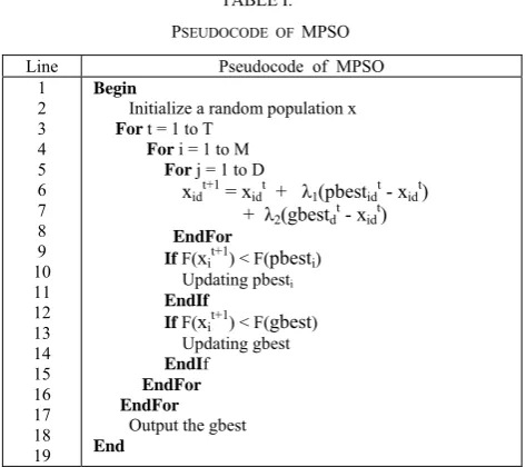
The main procedure of MPSO is shown in Table I:

TABLE I. PSEUDOCODE OF MPSO Line Pseudocode of MPSO

1 2 3 4 5 6 7 8 9 10 11 12 13 14 15 16 17 18 19 Begin

Initialize a random population x For t = 1 to T

For i = 1 to M

For j = 1 to D

xidt+1 = xidt + λ1(pbestidt - xidt)

+ λ2(gbestdt - xidt)

EndFor

If F(xit+1) < F(pbesti)

Updating pbesti

EndIf

If F(xit+1) < F(gbest)

Updating gbest EndIf

EndFor EndFor

Output the gbest

End

IV. SIMULATIONS AND COMPARISONS

In this section, we implement the simulations based on four benchmark problems to test the performances of the proposed MPSO for reliability-redundancy optimization problems. And we compared the MPSO with some other typical algorithms from the literatures.

A penalty function method is used to handle constrains, it is described as follows:

(6)

Where F(x) represents penalty function, f(x) represents objective function. gj(x), (j = 1, 2, …, p) represents the jth

constraint, and λ is a large positive constant which imposes penalty on unfeasible solutions, and it is named as penalty coefficient.

A. Series System

The series system [33] is shown as Figure 1:

Figure 1. Series system

This problem is formulated as follows:

m i 1 Z n , 1 ri 0 W )) 4 / n exp( n w ) n , r ( g C )) 4 / n exp( n ( ) r ln / 1000 ( ) n , r ( g V n v w ) n , r ( g .t . s ) n ( R ) n , r ( f Max i m 1 i i i i 3 m 1 i i i i i 2 m 1 i 2 i 2 i i 1 m 1

i i i

i ≤ ≤ ∈ ≤ ≤ ≤ = ≤ + − α = ≤ = = + = = β = =

∑

∏

， (7)

Where m is the number of subsystems, ni is the number

of components of subsystem i, Ri ( ni ) is the reliability of

subsystem i, f(r,n) is the reliability of the system; The wi

is the weight of each component in subsystem i, vi is the

1 2 3 4 5

∑

= λ + − = p 1 j

j(x)}

(4)

volume of each component in subsystem i; The ri is the

reliability of each component in subsystem i; The item

αi(-1000/lnri)βi is the cost of each component in

subsystem i, the parameters αi and βi is the constant

value(usually assume that have been given),1000 is the

task time of the components(it is commonly expressed in Tm); The V is the upper limit of total volume of the

system, C is the upper limit of total cost of the system, W is the upper limit of total weight of the system. The parameters for this problem are listed in TableII:

TABLE II.

THE PARAMETERS OF SERIES SYSTEM AND COMPLEX (BRIDGE) SYSTEM. Subsystem i 105_α

i βi wivi2 wi V C W

1 2.33 1.5 1 7 110 175 200

2 1.450 1.5 2 8

3 0.541 1.5 3 8

4 8.050 1.5 4 6

5 1.950 1.5 2 9

The proposed algorithm runs 50 times for this problem

independently, and the statistical results are computed and compared with other methods in other literatures. The list is as follows:

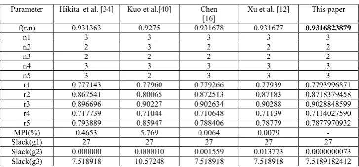
TABLE III.

BEST RESULTS COMPARISON ON SERIES SYSTEM

Parameter Hikita et al. [34] Kuo et al.[40] Chen [16]

Xu et al. [12] This paper

f(r,n) 0.931363 0.9275 0.931678 0.931677 0.9316823879

n1 3 3 3 3 3 n2 2 3 2 2 2 n3 2 2 2 2 2 n4 3 3 3 3 3 n5 3 2 3 3 3

r1 0.777143 0.77960 0.779266 0.77939 0.7793996871

r2 0.867541 0.80065 0.872513 0.87183 0.8718379458

r3 0.896696 0.90227 0.902634 0.90288 0.9028848599

r4 0.717739 0.71044 0.710648 0.71139 0.7114027590

r5 0.793889 0.85947 0.788406 0.78779 0.7877970932

MPI(%) 0.4653 5.769 0.0064 0.0079 -

Slack(g1) 27 27 27 27 27

Slack(g2) 0.000000 0.000010 0.001559 0.013773 0.0000000073 Slack(g3) 7.518918 10.57248 7.518918 7.518918 7.5189182412

Note: (1) the bold values denote the best values of those obtained by all the algorithms. (2) MPI (%) = (f − fother)/ (1 − fother ).

(3)Slack is the unused resources.

It can be seen from Table III, that the best results reported by Hikita et al. , Hsieh et al. , Chen and Xu et al. were 0.931363, 0.9275, 0.931678 and 0.9316823879 for the series system respectively. The result obtained by MPSO is better than the above four best solution, and the corresponding improvements made by the presented method are 0.4653%, 5.769% , 0.0064% and 0.0079% respectively.

B. Series-parallel System

The Series-parallel system[34] is shown as Figure 2:

Figure 2. Series-parallel system

) R )) R 1 )( R 1 ( 1 ( 1 )( R R 1 ( 1 ) n , r ( f

Max = − − 1 2 − − − 3 − 4 5 (8)

The constraints are the same as series system. The parameters for this problem are listed in Table IV:

TABLE IV.

THE PARAMETERS OF SERIES-PARALLEL SYSTEM.[34] Subsystem i 105_α

i βi wivi2 wi V C W

1 2.500 1.5 2 3.5 180 175 100

2 1.450 1.5 4 4.0

3 0.541 1.5 5 4.0

4 0.541 1.5 8 3.5

5 2.100 1.5 4 4.5

The proposed algorithm runs 50 times for this problem independently. Then the statistical results are calculated

and compared. The list is as follows:

1 2

3

4

(5)

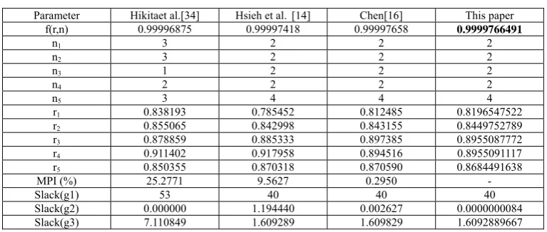
TABLE V.

BEST RESULTS COMPARISON ON SERIES PARALLEL SYSTEM

Parameter Hikitaet al.[34] Hsieh et al. [14] Chen[16] This paper f(r,n) 0.99996875 0.99997418 0.99997658 0.9999766491

n1 3 2 2 2

n2 3 2 2 2

n3 1 2 2 2

n4 2 2 2 2

n5 3 4 4 4

r1 0.838193 0.785452 0.812485 0.8196547522

r2 0.855065 0.842998 0.843155 0.8449752789

r3 0.878859 0.885333 0.897385 0.8955087772

r4 0.911402 0.917958 0.894516 0.8955091117

r5 0.850355 0.870318 0.870590 0.8684491638

MPI (%) 25.2771 9.5627 0.2950 -

Slack(g1) 53 40 40 40

Slack(g2) 0.000000 1.194440 0.002627 0.0000000084

Slack(g3) 7.110849 1.609289 1.609829 1.6092889667

It can be seen from TableV, that the best results reported by Hikita et al., Hsieh et al. and Chen were 0.99996875, 0.99997418 and 0.99997658 for the series– parallel system respectively. The result obtained by MPSO is better than the above three best solution, and the corresponding improvements made by the presented method are 25.2771%, 9.5627% and 0.2950% respectively.

C. Complex (bridge) System

The complex (bridge) system[35] is shown as Figure 3:

Figure 3. Complex (bridge) system

5 4 3 2 1 5 4 3 2 5 4 3 1

5 4 2 1 5 3 2 1 4 3 2 1

5 3 2 5 4 1 4 3 2 1

R R R R R 2 R R R R R R R R

R R R R R R R R R R R R

R R R R R R R R R R ) n , r ( f Max

+ −

−

− −

−

+ +

+ =

(9)

The constraints are the same as series system. The parameters for this problem are listed in TableII:

The presented algorithm runs 50 times for this problem independently, and the statistical results are calculated and compared. The list is as follows:

TABLE VI.

BEST RESULTS COMPARISON ON COMPLEX (BRIDGE) SYSTEM

Parameter Hikita. et al.[34]

Hsieh et al. [14]

Chen [16] Coelho [22] This paper

f(r,n) 0.9997894 0.99987916 0.99988921 0.99988957 0.9998896376

n1 3 3 3 3 3

n2 3 3 3 3 3

n3 2 3 3 2 2

n4 3 3 3 4 4

n5 2 1 1 1 1

r1 0.814483 0.814090 0.812485 0.826678 0.8280816704

r2 0.821383 0.864614 0.867661 0.857172 0.8578118137

r3 0.896151 0.890291 0.861221 0.914629 0.9142411461

r4 0.713091 0.701190 0.713852 0.648918 0.6481547109

r5 0.814091 0.734731 0.756699 0.715290 0.7040665038

MPI (%) 47.5962 8.6706 0.3860 0.0612 -

Slack(g1) 18 18 18 5 5

Slack(g2) 1.854075 0.376347 0.001494 0.000339 0.0000000087

Slack(g3) 4.264770 4.264770 4.264770 1.560466 1.5604662888

It can be seen from Table VI, that the best results reported by Hikita et al., Hsieh et al., Chen and Coelho were 0.9997894, 0.99987916, 0.99988921 and 0.99988957 for the complex (bridge) system respectively.

The result obtained by MPSO is better than the above four best solution, and the corresponding improvements made by the presented method are 47.5962%, 8.6706%, 0.3860% and 0.0612% respectively.

1 2

3 5

(6)

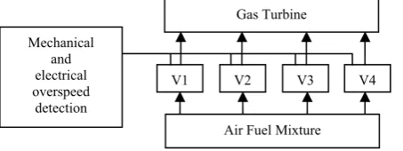
D. Overspeed Protection System

The problem is used to overspeed protection of a gas turbine. When the overspeed occurs, the system will be cut off. The overspeed protection system [36] is shown as Figure 4:

Figure 4. The overspeed protection system of a gas turbine

The control system can be viewed as an N-stage (N=4) mixed series-parallel systems. The model is formulated as follows:

+ −

+ =

= =

=

∈ −

≤ ≤

∈ ≤ ≤

≤ =

≤ +

⋅ =

≤ =

− − =

∑

∏

R r , 10 1 r 5 . 0

Z n , 10 n 0 . 1

W ) 4 / n exp( n w ) n , r ( h

C )] 4 / n exp( n [ ) r ( C ) n , r ( h

V n v ) n , r ( h . t. s

] ) r 1 ( 1 [ ) n , r ( f Max

i 6 i

i i

m

1 i

i i i 3

i i

m

1

i i

2

m

1 i

2 i i 1

m

1 i

n i i

(10)

Here C(r ) ( T /ln r ) i i i

i = α − β , T is the task time of the components, the parameters αi and βi is the same as

series system.

The parameters for this problem are listed in Table VII:

TABLE VII.

THE PARAMETERS OF OVERSPEED PROTECTION SYSTEM. Subsystem i 105

αi

βi vi wi V C W T

1 1 1.5 1 6 250 400 500 1000

2 2.3 1.5 2 6

3 0.3 1.5 3 8

4 2.3 1.5 2 7

The proposed algorithm runs 50 times for this problem

Independently, and the statistical results are calculated and compared. The list is as follows:

TABLE VIII.

BEST RESULTS COMPARISON ON OVERSPEED PROTECTION SYSTEM

Parameter Yokota et al. [35] Dhingra[36] Chen[16] Coelho [22] This paper

f(r,n) 0.999468 0.99961 0.999942 0.999953 0.9999546747

n1 3 6 5 5 5

n2 6 6 5 6 6

n3 3 3 5 4 4

n4 5 5 5 5 5

r1 0.965993 0.81604 0.903800 0.902231 0.9016123483

r2 0.760592 0.80309 0.874992 0.856325 0.8499199719

r3 0.972646 0.98364 0.919898 0.9481450 0.9481399512

r4 0.804660 0.80373 0.890609 0.883156 0.8882260306

MPI (%) 91.4802 88.3781 21.8529 3.5632 -

Slack(g1) 92 65 50 55 55

Slack(g2) 70.733576 0.064 0.002152 0.975465 0.0000001522

Slack(g3) 127.583189 4.348 28.803701 24.801882 24.8018827221

It can be seen from Table VIII, that the best results reported by Yokota et al., Dhingra, Chen and Coelho were 0.999468, 0.99961, 0.999942 and 0.999953 for the overspeed protection system respectively. The result is better than the above four best solution, and the corresponding improvements made by the presented

method are 91.4802%, 88.3781%, 21.8529% and 3.5632% respectively.

The statistical results comparison of four benchmark problems are listed in TableIX, including the best results(Best), the worst results(Worst), the mean results (Mean)and standard deviation(SD).

TABLE IX.

STATISTICAL RESULTS COMPARISON ON SERIES SYSTEM

Algorithm Best Worst Mean SD

ABC[37] 0.931682 NA 0.930580 8.14E-04

IA[17] 0.931682340 NA 0.931682222 1.3E-14 MPSO 0.9316823879 0.9315359727 0.9316621658 3.84E-05

Gas Turbine

Air Fuel Mixture V1

Mechanical and electrical overspeed

detection

(7)

TABLE X.

STATISTICAL RESULTS COMPARISON ON SERIES PARALLEL SYSTEM

ABC[37] 0.99997731 NA 0.99997517 2.89E-06

CDEHS[29] 0.99997665 0.99996475 0.99997365 4.3E-06 MPSO 0.9999766491 0.9999765280 0.9999766174 3.87E-08

TABLE XI.

STATISTICAL RESULTS COMPARISON ON COMPLEX (BRIDGE) SYSTEM

ABC[37] 0.99988962 NA 0.99988362 1.03E-05

PSO [22] 0.99988957 0.99987750 0.99988594 6.9E-07 EGHS[20] 0.99988960 0.99982887 0.99988263 1.6E-05 CDEHS[29] 0.99988964 0.99988931 0.99988940 1.9E-07

MPSO 0.9998896376 0.9998881138 0.9998891423 4.31E-07

TABLE XII.

STATISTICAL RESULTS COMPARISON ON OVERSPEED PROTECTION SYSTEM

GA[35] 0.999468 0.989207 0.9954507 NA

IA[16] 0.999942 NA NA NA

ABC[37] 0.9999550 NA 0.9999487 9.24E-06

PSO [22] 0.999953 0.999638 0.999907 1.1E-05

EGHS[20] 0.99995463 0.99985315 0.99993588 2.2E-05 CDEHS[29] 0.999955 0.999825 0.999926 2.9E-05 MPSO 0.9999546747 0.9999545194 0.9999546497 4.23E-08

It can be clearly seen from Table IX that the algorithm proposed in this paper have best value in terms of the best results and better value in terms of the mean results.

From Table X, it can be seen that the MPSO can get best value about the best results and the worst results, and get better value about the average results.

Through the comparison in Table XI, we can see that the MPSO can find better value than ABC, PSO and EGHS in terms of performance indexes, and get the same good value as CDEHS on the best results.

In Table XII, it is obvious that the MPSO has been got the best value of all the performance indexes. Moreover this method has small standard deviation for solving four benchmark problems. These demonstrate that the DEABM is effective and robust for solving reliability redundancy allocation.

V. CONCLUSIONS AND FUTURE WORK

In this paper, we proposed a modified particle swarm optimization (MPSO) algorithm to solve the reliability– redundancy optimization problems. The MPSO modifies the strategy of generating new position of particles. For each generation solution, the flight velocity of particles is removed. Whereas the new position of each particle is generated by using difference strategy. In addition, an adaptive parameter λ1 is used in MPSO. It can ensure

diversity of feasible solutions to avoid premature convergence. Simulation experiments based on four benchmark problems and compared with some algorithms in literatures. The results showed that the MPSO algorithm was effective, efficient and performed better on finding better feasible solutions than the other methods in the literatures. The future work is to improve the performance of the algorithm further and applied it to solve more complex constrained optimization problems.

REFERENCES

[1] W. Kuo, and V.R. Prasad, “An annotated overview of system-reliability optimization,” IEEE Transaction on Reliability, vol. 49 (2), pp. 176–187, 2000.

[2] M.S. Chern, “On the computational complexity of reliability redundancy allocation in a series system, ” Operations Research Letters, vol. 11, pp. 309–315, 1992. [3] K.B. Misra, and J. Sharma, “A new geometric

programming formulation for a reliability system,” International Journal of Control, vol. 18, pp. 497–503, 1973.

[4] Z. Y. Wu et al., “A new auxiliary function method for general constrained global optimization,” Optimization, vol. 62, No. 2, pp. 193–210, 2013.

[5] F.S. Hiller, and G.J. Lieberman, “An Introduction to Operations Research,” McGraw-HillCo, New York, 1995. [6] Y. Nakagawa, and S. Miyazaki, “Surrogate constraints

algorithm for reliability optimization problems with two constraints,” IEEE Transaction on Reliability, vol. R 30, pp. 175–180, 1981.

[7] K.S. Park, “Fuzzy apportionment of system reliability,” IEEE Transactions on Reliability, vol. R 36, pp. 129–132, 1987.

[8] Y.C. Hsieh, “A linear approximation for redundant reliability problems with multiple component choices,” Computers and Industrial Engineering, vol. 44, pp. 91–103, 2003.

[9] V.R. Prasad, and W. Kuo, “Reliability optimization of coherent system,” IEEE Trans. Reliab, vol. 49, pp. 323– 330, 2000.

[10]Ho-Gyun Kim, Chang-OK Bae, and Dong-Jun Park, “Reliability-redundancy optimization using simulated annealing algorithms,” Journal of Quality in Maintenance Engineering, vol. 12(4), pp. 354-363, 2006.

(8)

[12]Z. Xu, W. Kuo, and H.H. Lin, “Optimization limits in improving system reliability,” IEEE Transactions on Reliability, vol. 39, pp. 51–60, 1990.

[13]Y.C. Liang, and Y.C. Chen, “Redundancy allocation of series–parallel systems using a variable neighborhood search algorithm,” Reliability Engineering and System Safety, vol. 92, pp. 323–331, 2007.

[14]Yi-Chih Hsieh, Ta-Cheng Chen, and Dennis L. Bricker, “Genetic algorithms for reliability design problems,” Microelectronics Reliability, vol. 38, pp. 1599-1605, 1998. [15]P.S. You, and T.C. Chen, “An efficient heuristic for

series–parallel redundant reliability problems,” Computers and Operations Research, vol. 32(8), pp. 2117–2127, 2005. [16]Ta-Cheng Chen, “IAs based approach for reliability

redundancy allocation problems,” Applied Mathematics and Computation, vol. 182(2), pp. 1556-1567, 2006. [17]Y.-C. Hsieh, and P.-S. You, “An effective immune based

two-phase approach for the optimal reliability–redundancy allocation problem,” Applied Mathematics and Computation, vol. 218, pp. 1297–1307, 2011.

[18]D.W. Coit, and A.E. Smith, “Reliability optimization of series–parallel systems using a genetic algorithm, ” IEEE Transactions on Reliability, vol. 45, pp. 254–260, 1996.

[19]Dexuan Zou, Liqun Gao, Jianhua Wu, Steven Li, and Yang Li, “A novel global harmony search algorithm for reliability problems,” Computers & Industrial Engineering, vol. 58, pp. 307–316, 2010.

[20]Dexuan Zou, Liqun Gao, Steven Li, and Jianhua Wu, “An effective global harmony search algorithm for reliability problems,” Expert Systems with Applications, vol. 38, pp. 4642–4648, 2011.

[21]A.E.M. Zavala, E.R.V. Diharce, and A.H. Aguirre, “Particle evolutionary swarm for design reliability optimization,” Lecture Notes in Computer Science 3410, Presented at the Third International Conference on Evolutionary Multi-Criterion Optimization, Guanajuato, Mexico, pp. 856–869, March 9–11, 2005.

[22]Leandro dos Santos Coelho, “An efficient particle swarm approach for mixed-integer programming in reliability– redundancy optimization applications,” Reliability Engineering and System Safety, vol. 94, pp. 830–837, 2009.

[23]Shi-Ming Chen, Ali Sarosh, and Yun-Feng Dong, “Simulated annealing based artificial bee colony algorithm for global numerical optimization,” Applied Mathematics and Computation, vol. 219, pp. 3575–3589, 2012.

[24]Mohamed Ouzineb, Mustapha Nourelfath, and Michel Gendreau, “Tabu search for the redundancy allocation problem of homogenous series–parallel multi-state systems, ” Reliability Engineering and System Safety, vol. 93, pp. 1257–1272, 2008.

[25]Nabil Nahas, Mustapha Nourelfath, and Daoud Ait-Kadi, “Coupling ant colony and the degraded ceiling algorithm for the redundancy allocation problem of series–parallel systems, ” Reliability Engineering and System Safety, vol. 92, pp. 211–222, 2007.

[26]Manju Agarwal, and Vikas K. Sharma, “Ant colony approach to constrained redundancy optimization in binary systems,” Applied Mathematical Modelling, vol. 34, pp. 992–1003, 2010.

[27]Ling Wang, and Ling-po Li, “A coevolutionary differential evolution with harmony search for reliability-redundancy optimization,” Expert Systems with Applications, vol. 39, pp. 5271–5278, 2012.

[28]Nima Safaei, Reza Tavakkoli-Moghaddamb, and Corey Kiassat, “Annealing-based particle swarm optimization to

solve the redundant reliability problem with multiple component choices,” Applied Soft Computing, vol. 12, pp. 3462–3471, 2012.

[29]Leonardo Dallegrave Afonso, Viviana Cocco Mariani, and Leandro dos Santos Coelho, “Modified imperialist competitive algorithm based on attraction and repulsion concepts for reliability-redundancy optimization,” Expert Systems with Applications, vol. 40, pp. 3794–3802, 2013. [30]J. Kennedy, and R. Eberhart, “Particle Swarm

Optimization,” Proceedings of IEEE International Conference on Neural Networks IV, pp. 1942–1948, 1995. [31]W-N. Chen, and J. Zhang, “A novel set-based particle

swarm optimization method for discrete optimization problem,” IEEE Transactions on Evolutionary Computation, 14 (2), PP. 278–300, 2010.

[32]Z-H. Zhan, J. Zhang, Y. Li, and Y-H Shi, “Orthogonal Learning Particle Swarm Optimization,” IEEE Transactions on Evolutionary Computation, 15 (6): 832– 847, 2011

[33]K. Gopal, K. Aggarwal, and J.S. Gupta, “An improved algorithm for reliability optimization,” IEEE Trans. Reliab, vol. 27, pp. 325–328, 1978.

[34]M. Hikita, Y. Nakagawa, and H. Harihisa, “Reliability optimization of systems by a surrogate constraints algorithm,” IEEE Trans. Reliab, vol. 41, pp. 473–480, 1992.

[35]T. Yokota, M. Gen, and Y.X. Li, “Genetic algorithm for non-linear mixed integer programming problems and its applications,” Comput. Ind. Eng, vol. 30, pp. 905–917, 1996.

[36]Anoop K. Dhingra, “Optimal Apportionment of Reliability & Redundancy in Series Systems Under Multiple Objectives,” IEEE Transactions on Reliability, vol. 41(4), pp. 576-582, 1992.

[37]W.C. Yeh, and T.J. Hsieh, “Solving reliability redundancy allocation problems using an artificial bee colony algorithm,” Comput. Oper. Res, vol. 38, pp. 1465–1473, 2011.

[38]Harish Garg, and S.P. Sharma, “Multi-objective reliability-redundancy allocation problem using particle swarm optimization,” Computers & Industrial Engineering, vol. 64, pp. 247–255, 2013.

[39]Chunping Hu, Cuifang Wang, and Xuefeng Yan, “A self-adaptive differential evolution algorithm based on ant system with application to estimate kinetic parameters,” Optimization, vol. 61(1), pp. 99–126, January 2012. [40]Kuo W, Hwang CL and Tillman FA, “A note on heuristic

methods in optimal system reliability,” IEEE Transactions on Reliability, vol. R-27(5), pp. 320–324, 1978.

[41]Lino Costa et al., “An adaptive constraint handling technique for evolutionary algorithms,” Optimization, vol. 62(2), pp. 241–253, 2013.

Yubao Liu received M. Sc. from Changchun University of

Science and Technology in 2004. He is a doctoral student in Jilin University now and his research interests are mainly focused on system reliability, stochastic optimization, and artificial intelligence.

Guihe Qin received M. Sc. and Sc. D. degrees in