A simple multiband approach for solving frequency dependent problems in numerical time domain methods

A simple multiband approach for solving 

frequency dependent problems in 

numerical time domain methods

Sheaffer, J, Fazenda, BM, Murphy, DT and Angus, JAS

Title

A simple multiband approach for solving frequency dependent problems in 

numerical time domain methods

Authors

Sheaffer, J, Fazenda, BM, Murphy, DT and Angus, JAS

Type

Conference or Workshop Item

URL

This version is available at: http://usir.salford.ac.uk/id/eprint/16555/

Published Date

2011

USIR is a digital collection of the research output of the University of Salford. Where copyright 

permits, full text material held in the repository is made freely available online and can be read, 

downloaded and copied for non­commercial private study or research purposes. Please check the 

manuscript for any further copyright restrictions.

A simple multiband approach for solving

frequency dependent problems in numerical time

domain methods

Jonathan D. Sheaffer, Bruno M. Fazenda, Jamie A. S. Angus

Acoustics Research Centre, University of Salford, Salford, UK.

Damian T. Murphy

Department of Electronics Engineering, University of York, York, UK.

Summary

With the rapid growth of computational power and recent advances in GP-GPU technology, numerical time domain methods are becoming increasingly popular for room acoustics applications due to their accuracy, simplicity and ease of implementation. However, in order to model realistic spaces one should consider boundary conditions and source directivity functions as empirically measured frequency dependent quantities. Previously suggested methods rely on performing time domain convolution or employing recursive filters at the boundaries of the domain. Although shown to be highly accurate, these formulations normally involve complex implementations which not only reduce the attractiveness of using such methods, but may also result in computationally expensive algorithms. In this paper we examine a straightforward approach for solving such frequency dependent problems at the expense of being able to run a single broadband simulation. Using the finite difference time domain (FDTD) method, a number of band-limited frequency independent simulations are initiated in intervals depending on the availability of empirical impedance and directivity data and the desired spectral resolution. Generated impulse responses are filtered according to their respective frequency bandwidths and summed to produce a single frequency dependent impulse response. Intermediate values are automatically interpolated based on the characteristics of the chosen post processing filters. Results are analysed and validated and agreement with theoretical models is shown.

PACS no. 43.55.Ka, 43.55.Br

1.

Introduction

Numerical time domain methods are a family of wave-based algorithms for time-iterative solutions of the acoustic wave equation, which can be utilized for simulation of a wide range of acoustic problems, including wave propagation in rooms. As these methods essentially reduce the governing partial differential equations to simple discrete difference-equations, they are considered simple to implement and very suitable for parallel solution. However, in order to model realistic spaces one

1_{(c) European Acoustics Association}

spectral resolution. Generated impulse responses are filtered according to their respective frequency bandwidths and summed to produce a single frequency dependent impulse response. This is especially practical due to the fact the most empirically measured data are given in the form of real-valued absorption coefficients in octave or third octave bands. With recent advances in GP-GPU applications in room acoustics [3], this approach also follows one of the key aspects of the GPU programming paradigm. With frequency independent formulations thread operation is inherently more unanimous than with frequency dependent formulations, due to the reduced complexity of the boundary update equations. Furthermore, this approach allows for a simple implementation of frequency-dependent sources, as with each individual simulation a different directivity patterns may be implemented in their natural frequency independent form. In this paper,

this ‘multi-pass’ approach is examined in terms of

its accuracy and computational costs for GPU implementation.

2.

Compact Explicit Schemes for the

Wave Equation

Whilst the proposed approach may be applicable to any time-iterative algorithm, in this study we have opted to follow a compact finite difference model recently formulated by Kowalczyk and van Walstijn [4], due to its flexibility and rigorous boundary model. According to their nomenclature the 2nd _{order acoustic wave equation is discretised}

as follows:

ߜ_௧ଶ_݌ȁ ௜ǡ௝ǡ௞

௡ _{ൌ ߣ}ଶ_ሾ൫ߜ

௫ଶ൅ ߜ௬ଶ൅ ߜ௭ଶ൯ ൅

ܽ൫ߜ௫ଶߜ௬ଶ൅ ߜ௬ଶߜ௭ଶ൅ ߜ௫ଶߜ௭ଶ൯ ൅

ܾߜ௫ଶߜ௬ଶߜ௭ଶሿ݌ȁ௜ǡ௝ǡ௞௡ (1)

Where p is the acoustic pressure calculated on a grid discretised by

݌ȁ_{௜ǡ௝ǡ௞}௡ ൌ

݌ሺݔǡ ݕǡ ݖǡ ݐሻȁ_{௫ୀ௜௑ǡ௬ୀ௝௑ǡ௭ୀ௞௑ǡ௧ୀ௡்} (2)

2_{(c) European Acoustics Association}

Where X is the spatial sampling period related to the temporal sampling period T by the Courant criterion ߣ ൌ ܿܶȀܺ. The difference operators are further given by

ߜ_௧ଶ_݌ȁ ௜ǡ௝ǡ௞

௡ _{ൌ ݌ȁ}

௜ǡ௝ǡ௞ ௡ାଵ_{െ ʹ݌ȁ}

௜ǡ௝ǡ௞

௡ _{൅ ݌ȁ}

௜ǡ௝ǡ௞ ௡ିଵ

ߜ_௫ଶ_݌ȁ ௜ǡ௝ǡ௞

௡ _{ൌ ݌ȁ}

௜ାଵǡ௝ǡ௞ ௡ _{െ ʹ݌ȁ}

௜ǡ௝ǡ௞

௡ _{൅ ݌ȁ}

௜ିଵǡ௝ǡ௞ ௡

ߜ௬ଶ݌ห_{௜ǡ௝ǡ௞}௡ ൌ ݌ȁ௜ǡ௝ାଵǡ௞௡ െ ʹ݌ȁ௜ǡ௝ǡ௞௡ ൅ ݌ȁ௜ǡ௝ିଵǡ௞௡

ߜ_௭ଶ_݌ȁ ௜ǡ௝ǡ௞

௡ _{ൌ ݌ȁ}

௜ǡ௝ǡ௞ାଵ ௡ _{െ ʹ݌ȁ}

௜ǡ௝ǡ௞

௡ _{൅ ݌ȁ}

௜ǡ௝ǡ௞ିଵ

௡ ₍₃₎

Choosing the free variables a and b in (1) (see [4] table I), and combining with the operators from (3), allows a derivation of a range of explicit finite difference equation which can be used to simulate wave propagation through the medium. At the outer faces, edges and corners of the grid, the governing equation is modified such that it would satisfy the boundary conditions defined by the wall impedance (see equations 38, 44, 45 in [4]). For frequency dependent boundary conditions, a digital impedance filter is introduced which can be designed based on any arbitrarily available data. For the multi-pass investigations used in this work, we have utilized a zero-order filter, essentially corresponding to a frequency independent formulation.

3.

Boundary Reflectance

3.1. Methodology

The goal of this experiment is to observe how the multi-pass approach is applied to boundary conditions. In this investigation we follow the methodology suggested in [5] to determine the frequency dependent numerical reflectance of a boundary. A three-dimensional domain of ͵͹͵ଷ

nodes corresponding to a physical volume of 4096 cubic meters is modeled using the interpolated wideband (IWB) scheme with the coefficients set to ܽ ൌ ͳȀͶǡ ܾ ൌ ͳȀͳ͸ǡ ߣ ൌ ͳ . The scheme is particularly useful for this experiment as it exhibits an effective bandwidth of up to the Nyquist limit [4]. As the computational domain is in the order of tens of millions of elements, the model is implemented on a GPU.

positioned at a -45 degrees angle and at 94 nodes radial distance from the wall, far enough to consider a plane wave assumption for most frequencies of interest. Boundary conditions are applied to the wall under investigation to imitate arbitrarily given real-valued impedance. The model is designed in such way that it can be terminated before reflections from other boundaries arrive at the receiver positions, effectively windowing the RIR to include only the desired reflection.

Simulation is initiated and stopped once the desired reflection from the wall under investigation has reached a receiver situated at a +45 degrees angle from the specular reflection point. The signal at the receiver ݔ_௧௢௧ሾ݊ሿ is recorded and includes the direct source and a reflection from the wall under investigation. Next, the wall under investigation is removed and the source signal is re-radiated essentially in a virtual free field. The signal ݔௗሾ݊ሿ is then collected at the

original receiving point containing only the direct part of the sound field. Similarly, a signal ݔ௠ሾ݊ሿ is

recorded at a mirror position (+135 degrees from the specular reflection point), which features both the propagation delay and other inherent modelling artifacts.

The signal carrying the numerical reflection, ݔ௥ሾ݊ሿ , is simply obtained by the difference

between the total sound field and the direct field:

ݔ௥ሾ݊ሿ ൌ ݔ௧௢௧ሾ݊ሿ െ ݔௗሾ݊ሿ (4)

The signal containing the theoretically expected reflectance is obtained by a scalar multiplication of the expected plane wave reflection coefficient and the mirror signal ݔ_௠ሾ݊ሿ.

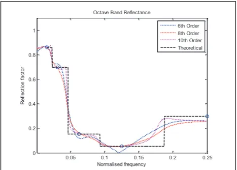
The entire operation is repeated with different boundary conditions for each octave-band; resulting in a set of frequency independent signals. The signals containing the theoretical reflectance and numerical reflectance are then each filtered according to their octave band centres and summed to form frequency dependent impulse responses. The octave band filters used are realised using 6th_,

8th _{and 10}th _{order Butterworth filters as shown in}

Figure 1. The frequency domain reflection factors are obtained by passing each of these signals

through a Hann window and performing frequency domain deconvolution between them.

3.2. Results

Figure 1 plots the theoretical vs. numerical reflection factors obtained from the experiment, using various filter orders. Nearest-neighbour interpolation is applied to the curve showing theoretical reflectance, originally given in octave bands.

Figure 1. Modelled reflectance (dotted) plotted against theoretical reflectance (dashed black and blue marks).

Although with the IWB scheme it is possible to model up to the frequency ͲǤͷ݂_௦, reliable results from this investigation are given only up to ͲǤʹͷ݂_௦. The reason for this is that the ͲǤͷ݂_௦ octave band includes frequencies essentially above both the Nyquist limit and the accuracy limit of the scheme.

It can be seen from Figure 1, that at least as far as reflection magnitude is concerned, the modelled reflectance follows its theoretical counterpart. It can also be noticed that any intermediate interpolation can be controlled by considering the structures of post-processing filters.

4.

Source Directivity

4.1. Methodology

The purpose of this experiment is to examine how frequency dependent source directivity can be implemented using the multi-pass approach. Using low complexity 1st order differential sources [6] radiation patterns were generated for the various

0.05 0.1 0.15 0.2 0.25

0 0.2 0.4 0.6 0.8 1

Normalised frequency

R

ef

lec

tion f

ac

tor

Octave Band Reflectance

frequency-band simulations, roughly corresponding to the directivity characteristics of a loudspeaker. The sources were injected into a 606x606 node grid using the 2D interpolated isotropic scheme [7], with the coefficients ܾ ൌ ͳȀ͸ǡ ߣ ൌ ඥͳȀʹ. This scheme is favorable for this sort of investigation as it is almost entirely isotropic up to ͲǤʹ݂_௦.

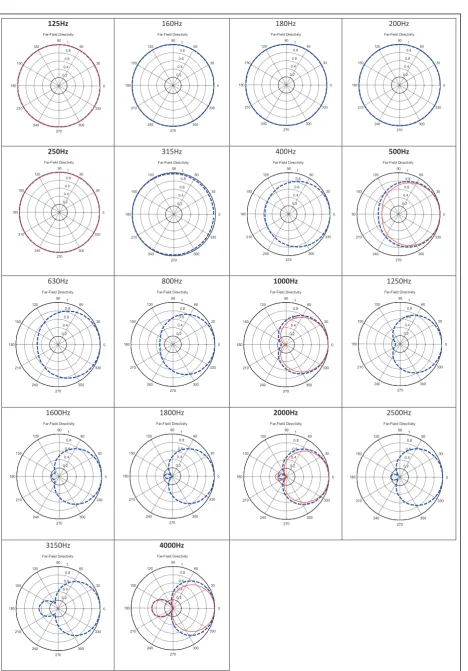
The source was situated at the centre of the domain and 72 receivers were placed around it in a radial distance corresponding to 178 nodes. Six simulation passes were conducted with data corresponding to the octave centres 125, 250, 500, 1000, 2000 and 4000 Hz. The obtained impulse responses were filtered using a 6th order Butterworth respectively. Data was then summed to form a set of frequency dependent RIRs, each corresponding to a different radial position around the source. This set of RIRs was further filtered into 1/3rd _{octave bands to examine how}

intermediate frequencies were interpolated in the filtering process.

4.2. Results

Figure 2 depicts 1/3rd octave frequency dependent source directivities generated using the multi-pass approach. In the corresponding octave bands the expected (theoretical) directivity is also shown. It can be seen that intermediate directivity patterns are automatically interpolated based on their neighboring values, very closely following their expected counterparts.

5.

Performance and Costs

5.1. Model

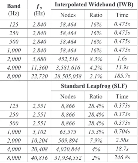
Two compact FDTD schemes were implemented: 1) the standard leapfrog scheme (SLF), also often referred to as the Kirchhoff Digital Waveguide Mesh (K-DWM) as it is the most commonly used and least computationally expensive; and 2) the interpolated wideband (IWB) scheme, as it provides the widest bandwidth and is the most computationally expensive. A 98m3 _{rectilinear room}

was modelled at different temporal and spatial sampling rates, as shown in Table I. Models were calibrated in terms of sampling rate such that both methods would cover the same theoretical bandwidth according to [4]. As absorption data is

normally given in octave bands from 125Hz to 8000Hz, 7 frequency independent simulations were executed to obtain an impulse response corresponding to 0.5 seconds long. Unlike the previous boundary reflectance investigation, here each simulation was band-limited, resulting in a coarse grid at low frequencies and a dense grid at higher frequencies. The purpose of this is to benchmark how long it takes to compute an entire 7-set of impulse responses whilst maintaining low computational costs. At very low frequency bands, a minimum update rate of 2000 Hz was maintained to preserve a minimum boundary-air node ratio.

5.2. GP-GPU Implementation

The models were accelerated using a general purpose graphics processing unit (GP-GPU), specifically the nVidia GTX 580 featuring the newly developed Fermi architecture. The hosting computer was based on an Intel Q6600 quad-core processor. Codes were written in C using nVidia’s

Compute Unified Device Architecture (CUDA) framework, and were implemented and optimized according to [8].

Band (Hz)

ࢌ࢙

(Hz)

Interpolated Wideband (IWB) Nodes Ratio Time

125 2,840 58,464 16% 0.475s 250 2,840 58,464 16% 0.475s 500 2,840 58,464 16% 0.475s 1,000 2,840 58,464 16% 0.475s 2,000 5,680 452,516 8.3% 1.6s 4,000 11,360 3,581,616 4.2% 13.9s 8,000 22,720 28,505,058 2.1% 185.7s

Standard Leapfrog (SLF) Nodes Ratio Time

125 2,551 8,866 28.4% 0.373s 250 2,551 8,866 28.4% 0.373s 500 2,551 8,866 28.4% 0.373s 1,000 5,102 65,575 15.3% 0.704s 2,000 10,204 509,894 7.9% 2.58s 4,000 20,408 4,020,844 4% 18.7s 8,000 40,816 31,934,552 2% 246.8s

Table I. Total amount of nodes, computation time and percentage of boundary nodes for different grid sizes

FORUM ACUSTICUM 2011 Sheaffer et al.: Multiband approach for frequency dependency 27. June - 1. July, Aalborg

Figure 2. Modelled directivity patterns in 1/3rd _{octave bands based on octave band data. Dashed blue lines denote} modelled dirctivity, solid red lines denote expected directivity.

.

125Hz 160Hz 180Hz 200Hz

250Hz 315Hz 400Hz 500Hz

630Hz 800Hz 1000Hz 1250Hz

1600Hz 1800Hz 2000Hz 2500Hz

3150Hz 4000Hz

FORUM ACUSTICUM 2011 Sheaffer et al.: Multiband approach for frequency dependency 27. June - 1. July, Aalborg

5.3. Results

The multiple octave band passes were benchmarked and results were summed to show the total computation time. Offline processing time required for filtering and summing the signals is neglected. The factor of the total computation time and the computation time of the grid at the highest investigated sampling rate, is regarded to as the increase in computational expense for turning the frequency independent problem into a frequency dependent one by means of the multi-pass approach. For both the IWB and SLF schemes the increase in computation time is roughly 9.4%, a small trade-off for the benefits of frequency dependency. As a crude comparison, Savioja [3] calculated a computational increase of 30%-70% using the single-pass approach, depending on the filter order required for the frequency dependent boundary. However, it should be borne in mind that these quantities strongly depend on the maximum update frequency of the grid as well as the geometry, boundary-air node ratio and memory management. Therefore, a more rigorous investigation is required in order to conclude whether the multi-pass approach is predominantly more efficient.

6.

Conclusions and Future Work

In this paper we have examined a multi-band approach for solving frequency dependency in numerical time domain methods. The proposed method can model frequency dependent boundary conditions as well as frequency dependent source functions, where intermediate band interpolation is controlled by the structures of the post processing filters. The method is very simple to implement and is computationally efficient.

However, the multi-pass approach has a few handicaps. First, it requires offline processing, hence cannot be used for real time applications. Also, to avoid spatial aliasing source functions are normally band-limited resulting in differently shaped excitation signals which cannot be straightforwardly summed. Therefore, unless oversampling is inherently required (resulting in the ability to maintain a constant source function shape), a single RIR cannot be simply obtained by

time domain summation. Alternatively, a frequency domain manipulation may be considered, requiring further signal processing. Another challenge is controlling the phase response of the system, as the frequency independent passes cannot account for complex impedance; whereas digital impedance filters can be designed to match both magnitude and phase. Nevertheless, for many applications this is not an issue as empirically measured impedance values are normally available in the form of real absorption coefficients. Future work will include a more comprehensive benchmark, and an investigation into time and frequency domain accuracy of the multi-pass approach in comparison to the single-pass method. Another important aspect that should be looked at, is how both methods compare from an auditory perceptual point of view.

Acknowledgements

The authors would like to thank Dr Konrad Kowalczyk for the fruitful discussions on boundary modelling.

References

[1] D. T. Murphy and M. Beeson, “The KW-boundary

hybrid digital waveguide mesh for room acoustics

applications,” IEEE Trans. Aud. Speech. Lang.

Proc., vol. 15, no. 2, p. 552, 2007.

[2] K. Kowalczyk and M. Van Walstijn, “Modeling

frequency-dependent boundaries as digital

impedance filters” J.Aud.Eng.Soc, vol. 56, no. 7/8,

p. 569–583, 2008.

[3] L. Savioja, “Real-Time 3D Finite-Difference Time-Domain Simulation of Mid-Frequency Room

Acoustics.”, 13th Intl. Conf. on DAFx, Sep. 2010.

[4] K. Kowalczyk and M. Van Walstijn, “Room acoustics simulation using 3-D compact explicit

FDTD schemes,” IEEE Trans. Aud. Speech. Lang.

Proc., no. 99, p. 1.

[5] K. Kowalczyk and M. van Walstijn, “Formulation

of Locally Reacting Surfaces in FDTD/K-DWM

Modelling of Acoustic Spaces,” Acta Acust. united

with Acustica, vol. 94, pp. 891-906, Nov. 2008.

[6] A. Southern and D. Murphy, “Low complexity

directional sound sources for finite difference time

domain room acoustic models,” in 126th Audio Eng.

Soc. Convention, 2009.

[7] K. Kowalczyk and M. Van Walstijn, “Wideband and isotropic room acoustics simulation using 2-D

interpolated FDTD schemes,” IEEE Trans. Aud.

Speech. Lang. Proc., vol. 18, no. 1, p. 78–89, 2009. [8] J. Sheaffer and B. Fazenda., “FDTD/K-DWM

Simulation of 3D Room Acoustics on General

Purpose Graphics Hardware” in Proc. Institute of