Classification of Stuck at Faults in Synchronous Sequential Circuits Using Artificial Neural Network

ISSN (e): 2250-3021, ISSN (p): 2278-8719

Vol. 08, Issue 11 (November. 2018), ||V (I) || PP 15-22

Classification of Stuck at Faults in Synchronous Sequential

Circuits Using Artificial Neural Network

G. Nithya

1

, M. Ramaswamy

2 1

(Department of Electronics and Communication Engineering, Annamalai University, India)

2_{(Department of Electrical Engineering, Annamalai University, India)}

Corresponding Author:G. Nithya

Abstract: The paper develops an artificial neural networks (ANNs) based procedure for classifying the stuck at

faults (SAF) in the primary output of the synchronous sequential circuits. It builds fault models based on back propagation (BPN) and the extreme learning machine algorithm (ELM) in an effort to process the circuit input– output measurements. It creates the fault dictionary by inserting single and two simultaneous stuck at faults in the circuit. The methodology explores different sizes of test vectors from the fault dictionary to classify the faults through a process of training with the circuit responses obtained from measuring and coding both the input and output signals. The results obtained with the serial adder as the CUT reveal that ANN can serve as an on line classifier for extraditing the occurrence of the SAFs. The comparative performance of the two algorithms show that the ELM based implementation results in faster learning and higher accuracy. The fundamental basis of the scheme enumerates a new dimensional scope for the role of ANN in classifying faults and allows it to claim a space in practical utilities.

Keywords: ANN, Back-propagation, ELM, Fault Classification, Stuck-at-Faults.

--- --- Date of Submission: 08-11-2018 Date of acceptance: 22-11-2018 --- ---

I.

INTRODUCTION

With increasing system complexity, shorter product lifecycles, lower production costs, and changing technologies, the need for intelligent tools at different stages of the product lifecycle becomes increasingly important. A system constitutes to be ―any aggregation of related elements that together form an entity of sufficient complexity and transcends to be impractical for treating the elements at the lowest level of detail1‖. The examples include automobiles, computers or electronic circuit boards and digital circuits built using very large scale integrated (VLSI) components.

The explosion of the integrated circuit technology brings with it challenges in the form of testing problems and associated issues. Besides it encounters a timing problem for testing the circuits even on the fastest automated equipment. Owing to the emergence of the microelectronic techniques, the scale of the electronic circuits increases and the structure becomes complex.

The mixed analogue and digital circuits experience similar difficulties and engages complications to determine a set of input test signals through which the output measurements shall provide a high degree of fault coverage. The fault diagnosis isolates the source(s) of a system malfunction, by collecting and analyzing the information on system status using measurements, tests, and other information sources in the form of observed symptoms.

The artificial neural networks (ANNs) find use in a wide variety of applications that extend over direct implementations in electronic and similar other domains and urge to exploit the parallelism implicit in the solution. An important consequence of implementing any circuit or device augurs the necessity of verifying that the device meets specifications (functional tests) and remain free from manufacturing defects (defect or fault tests). The functional tests assure that the system meets the desired specifications, but it shows to be ineffective for determining whether or not a circuit is defect free.

The ANNs have been shown to be a powerful means for fault classification and realizing a hardware that may be as fast as necessary to follow the changes of the system's response in real time. The application of neural net based techniques for fault classification appears to be promising particularly when dealing with problems involving poorly defined system models, noisy signals and non-linear behaviors.

the logic circuits represent the gates with more than two inputs using a hidden neuron. A fault diagnosis method based on artificial neural networks for multiple stuck at 0 and 1 fault has been discussed4. The method has been framed to convert the stuck at multiple faults into single fault by adding an additional gate.

The neural network models have been presented as a means of determining logical network satisfaction and as a means of determining test patterns for stuck-at faults5, without a learning phase but rather the dynamics of the neural network have been used as a means of computing inputs and outputs which yield minimum energy configurations.

A fault behavior model developed with a neural network concept in a novel way has been addressed in6. The neural network structure has been used to synthesize the faulty output of a circuit at a high-level of abstraction.

The test generation methods based on the networks models with Hopfield binary neural networks used to build the models has been envisaged in7.The Hopfield neural network8 model has been used in the single stuck-at fault test generation and constructs the constraint circuit of the single stuck-at fault circuit. The test vectors for the multiple stuck-at faults circuit have been obtained by applying artificial colony algorithm to solve the zero value of energy function of the constraint circuit‘s interface circuit.

A technique has been proposed for the use of ANNs for single and multiple stuck at fault classification. An efficient ANN architecture has been created with the ANN trained from the data derived using the circuit test data and offers significant improvement in multiple fault diagnosis9.

The artificial neural networks (ANNs) have been used for the classification of multiple faults after being trained with single stuck at failure information from a fault truth table (FTT)10. The table has been created to usually list the single-fault / No-fault conditions in the circuit against the resulting state of both internal and external nets.

The primary emphasis relates to exploring the use of both Back propagation and ELM for classifying single and multiple stuck at faults in synchronous sequential circuits through appropriate training algorithms. Finally the study orients to investigate the performance in terms of indices and illustrate the benefits of the use of the chosen methods.

II.

PROPOSED METHODOLOGY

Fault detection in digital circuits assumes significance to pave the way for fault-tolerant computing. The increasing complexity and very deep sub-micron technologies in digital circuits find the problem of fault detection, fault tolerance and test generation to be extremely difficult. The literature shows significant achievements in generating tests for combinational logic circuits under the assumption that there exists a greater probability for the occurrence of single faults of a stuck-at nature11,12,13.

The application of intelligence techniques to fault classification generates interest4,9,10,14,15,16,17 and remains typically applied to analog circuits. However the survey does not reflect any developments relating to synchronous digital circuits. The attempt encompasses to extend the analysis in16,17 to sequential circuits.

Fig.1: Circuit under test.

The choice of a serial binary adder as the CUT which performs 4-bit binary addition bit by bit and can be constructed with a full adder and one flip flop. The block diagram of the 4-bit serial adder seen from Fig.1 consists of two EXOR gates, two AND gates, one OR gate and one D flip flop with a purpose to add two single-bit inputs along with the carry. It yields two single-single-bit for the sum and carry outputs and adds each single-bit per clock cycle with the carry-in signal calculated from the previous carry-out signal.



1 in

 

1 2

 

2 in



out xC x x x C

C   

₍₁₎

in C x x sum

Z1( ) 1 2 ₍₂₎

Table no 1:State table for the serial binary adder. Present

state

Next state Output z1

x1x2 00 01 10 11 00 01 10 11

G G G G H 0 1 1 0

H G H H H 1 0 0 1

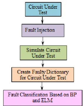
The flow chart shown in Fig. 2 outlines the proposed methodology governing the formulation of the classification of stuck at faults and measures introduced to identify the faults. The fault diagnosis approach based on fault dictionary generation gathers to be effective and the change of state transition caused in the circuit primary output under fault and fault free conditions leads to the fault classification. It contains the consecutive sets of binary circuit inputs and corresponding fault free and faulty outputs for each set of input combinations that can be used as the inputs to the ANN architecture in a serial form. Each entry in the fault dictionary in the form of sequences of the string arises by inserting single and multiple stuck at faults randomly in the CUT9.

Fig.2: Proposed methodology for fault classification.

The CUT in Fig.1 includes a fault site on each branch of the circuit and on each input and output of the gates for a total of 7 fault sites. However Sa0 and Sa1 faults can be injected in the 7 fault sites (7 × 2 = 14) and creates (14 + 1) × 256 = 3840 fields in the fault dictionary as shown in Table no 2 where 14 refers to the number of different faults that can be injected, 256 the number of different inputs for the CUT, and the extra 1 added to 14 to account for the output in the absence of a fault. Therefore the fault dictionary contains (14 +1) separate input patterns for the single fault and (84+1) input patterns for the double fault and the plus one for the fault free input pattern.

Table no2: Fault dictionary for serial binary adder,first 1792 injected fault fields show stuck-at-0 for all 7 different fault sites and second 1792 injected fault fields show stuck-at-1 for all 7

different fault sites.

Field Input of the circuit Fault injection Faulty output of the circuit

1 00000000 Stuck at ‗0‘at pt‗1‘ 0000

: .

: .

: .

: .

17 00010000 Stuck at ‗0‘at pt‗1‘ 0000

18 00010001 Stuck at ‗0‘at pt‗1‘ 0001

: .

: .

: .

256 11111111 Stuck at ‗0‘ at pt‗1‘ 1111 :

.

: .

: .

: .

259 00000010 Stuck at ‗0‘ at pt‗2‘ 0000

260 00000011 Stuck at ‗0‘ at pt‗2‘ 0000

: .

: .

: .

: .

511 11101111 Stuck at ‗0‘ at pt‗2‘ 1111

: .

: .

: .

: .

1540 00100110 Stuck at ‗0‘ at pt‗6‘ 0010

1541 00100111 Stuck at ‗0‘ at pt‗6‘ 0011

: .

: .

: .

: .

2064 00010000 Stuck at ‗1‘ at pt‗1‘ 1111

2065 00010001 Stuck at ‗1‘ at pt‗1‘ 0000

: .

: .

: .

: .

3839 11111110 Stuck at ‗1‘ at pt‗7‘ 1111

3840 11111111 Stuck at ‗1‘at pt‗7‘ 1110

The Table no 2 shows the separate input pattern formed by the sequences of the string of the possible ‗input‘ and ‗output‘ combinations for the different fault sites. The scheme exults the use of two different types of data derived using a C program corresponding to all possible input combinations and 50% of possible input combinations randomly in the fault dictionary.

The training of the ANN using back propagation (BP) algorithm with single fault information from the fault dictionary enables to test its ability to classify both single and multiple faults. It is a multilayer artificial neural network containing input layer, hidden layer and the output layer.

The procedure extends to classify the faults using a second model based on machine learning called Extreme Learning Machine (ELM) with lower time consumption and ease of operation. It not being sensitive to trade-off parameters enjoys good classification performance without the optimization of trade-off parameters in compressing the sampled space. The ELM provides better generalization performance at a faster learning speed with less human intervention and exhibits a very high capability to resolve problems of data regression and classification.

The ELM offers a single hidden layer feed forward neural network learning algorithm that can randomly chooses hidden nodes and determines the output weights connected to the hidden neuron in the output of the network analytically. It claims its use to several benchmarking problems and in many cases provides results that remain a thousand times faster than the traditional learning algorithms18.

The Fig. 3 shows the general ELM architecture with a single hidden layer where Xi and Ojrepresents the input and output nodes of the network and βi the weight connecting the hidden layer and the output node.

Fig.3: ELM architecture.

For a data set with N samples (xi, ti),

It carries out the classification problem through SLFN with Ñ hidden nodes and activation function g(x). The output nodes are linear and the output Oj can be expressed as in Eqn. (3):

 

x g



wx b



o for j N

g _{i i j i j}

N i i j i N i

i 1,2,...

~ 1 ~ 1    





 





(3) Where Wi 



Wi1,Wi2,...,Win



Trelate to the weights betweenthe input nodes and the j

th

hidden node,



i i im



T

i 1,2,...,

 

forms the output weight vector existing between the hidden layer and the output layer and bi the threshold of the ith hidden node. The network can approximate the given problem using Eqn.(4)



wx b



t for j N

g_{i i j i j}

N

i

i 1,2,...

~ 1   







(4) The above N equations can be written as in Eqn. (5)

T

H



 ₍₅₎

Where

















                        N N N N N N b x w g b x w g b x w g b x w g H ~ ~ 1 1 1 ~ 1 1 1 ... . . . ...                      T N ~ T 1 . . .                         T N T 1 . . . t t T

Given a training setD





Xi,ti



:Xi Rn,tiR,i1,2...N



, the number of hidden nodes and hidden node activation functions following steps explain the ELM algorithm.

Step 1:Random assignments of the weights between the hidden nodes and the input nodes wiand the bias of the hidden nodes.

Step 2: Calculation of the hidden layer output matrix.

Step 3: Calculation of the output weight β using: β = H†T

Where H† defines the generalized Moore-Penrose inverse matrix and the output weight gives the smallest norm least squares solution for the linear system to obtain the unique solution.

The flow diagram in Fig. 4 reflects to acquire randomly the training and testing samples normalized in the range -1 to 1from the fault dictionary in the ratio that seventy five percentages of data serve the process of training and the remaining twenty five percentages of data for testing.

The input weights and the bias of hidden neurons generated randomly allow the calculation of the hidden layer output matrix based on the activation function and compute the output weight from the pen-rose inverse of a hidden layer matrix and the target.

III.

RESULTS AND DISCUSSION

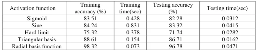
The ELM algorithm involves five input parameters in the form of training set, testing set, parameter to determine regression or classification, hidden nodes, and activation function. It engages five different activation functions that include sigmoid, sine, hard limit, triangular basis and radial basis functions. The performance measures of the varied activation functions indicate that the radial basis activation function produces the optimum performance compared to the other activation function because it inherits a better misclassification and compressing property as seen from Table no 3.

Table no3:Performance comparison of ELM with different activation functions.

The number of input neurons with possible input combinations and 50% of input combinations for the serial binary adder as the CUT turn out to be 3072and 1536 for single and double respectively. The number of neurons in the: hidden layer amount to 1025 and 512 for single and double fault respectively. The number of neurons in the output layer equals the number of possible single faults along with the fault free case in the circuit, which relates to 15 neurons for single and 85 neurons for double faults.

A set of 3840 x 8 samples from the fault dictionary with 2560 x 8 samples used for training and 1280 x 8 sample for testing the network constitute as inputs to both the ELM and back propagation methods for fault classification. It compares the performance of ELM algorithm with that of the BP-NN using confusion matrix, which contains information about the actual and predicted class. The matrix describes the possible outcomes of the result that include the True Positive (TP), True Negative (TN), False Positive (FP) and False Negative (FN). The symbol TP stands for the faults which occur and TN for those which do not occur. Similarly FP If the procedure identifies the faults when they actually do not occur and FN when the faults actually occur. The Eqns. (6)-(10) define indices that include the accuracy, sensitivity, specificity, error, and precision for analyzing the performance of the classification process.

FN FP TN TP

TN TP Accuracy

  

 

(6)

FN FP TN TP

FN FP Error

  

 

(7)

FN TP

TP y

Sensitivit

 

(8)

FP TN

TN y Specificit

 

(9)

Precision TP FP TP

 

(10) Activation function Training

accuracy (%)

Training time(sec)

Testing accuracy

(%) Testing time(sec)

Sigmoid 83.51 0.428 82.28 0.0312

Sine 84.24 0.831 83.32 0.0415

Hard limit 75.32 0.378 71.74 0.0282

Triangular basis 88.61 0.154 86.71 0.0162

Table no 4: Performance comparison of BP-NN and ELM for classifying single fault and double faults with all possible input combination

Table no5: Performance comparison of BP-NN and ELM for classifying single fault and double faults with 50% possible input combination.

The performance of BP-NN and ELM algorithm for classifying single and double stuck-at-faults in synchronous circuits are analysed and the parameter such as accuracy, error, precision, sensitivity, and specificity are tabulated in Table no. 4 and 5 for all and 50% possible input combination. The comparison between BP-NN and ELM is carried out and the result shows that ELM provides better performance in all aspects.

IV.

CONCLUSION

The theory of BP NN and ELM has been sought to formulate a fault classification technique for synchronous sequential circuit with serial binary adder as the CUT. The formulation has been laid to address both Sa0 and Sa1 faults in single and multiple forms on the interconnect lines. The training procedure has been enlivened with the data derived from circuit test vectors to evolve a compact, flexible and efficient ANN architecture with a focus to provide significant improvement in multiple fault classification. The results have been ordained to explain a faster learning and offer a higher accuracy for the ELM algorithm over the BP NN. The findings have been projected to claim a space for the use of AI techniques and accomplish an on-line fault classification mechanism for use in real world systems.

REFERENCES

[1] Simpson WR, Sheppard JW. System test and diagnosis. 1994; Boston, MA: Kluwer.

[2] Nicolaidis M, Zorian Y. On-line testing for VLSIA—compendium of approaches. J. Electron. Testing: Theory Application. 1998; 12: 7-20.

[3] Zhang Z, Mcleod, RD. Pedrycz W. A neural network algorithm for testing stuck-open faults in CMOS combinational circuits. Journal of Electronic Testing: Theory and Application. 1993; 4(3): 225 -235. [4] Zhao Y, Li Y. A multiple faults test generation algorithm based on neural networks and chaotic searching

for digital circuits. International Conference on Computational Intelligence and Software Engineering, 2010; 1–3.

[5] Chakradhar ST, Bushnell ML, Agrawal VD, Toward massively parallel automatic test generation. IEEE Trans. CAD. 1990; 9: 981-994.

[6] Zeynab M. Jean-Francois B, Yvon S. Modeling the faulty behaviour of digital designs using a feed forward neural network based approach. IEEE International Symposium on Circuits and Systems. 2015; 1518 – 1521.

[7] Ortega J, Prieto A, Lloris A, Pelayo F.J. Generalized Hopfield neural network for concurrent testing. IEEE Trans. on Computer, 1993; 42(8): 898-911.

[8] Bin XJ, Zhi L. The Application of Neural networks in the simulation-based test generation algorithm for hybrid circuits. Journal of Circuits and Systems. 2001; 6(4): 109-110.

[9] AL-Jumah AA, Arslan T. Artificial neural network based multiple fault Diagnosis in digital circuits. Proceedings of the IEEE International Symposium on Circuits and Systems. 1998; 2: 304 – 307.

[10] Arslan T, AL-Jumah A. A compact artificial neural network approach for multiple fault location in digital circuits. Electronics Letters. 1997; 33:1801-1803.

Performance measures

BP-NN ELM

Single fault Double Fault Single fault Double Fault

Accuracy (%) 94.1 92.94 100 98.82

Error(%) 5.88 7.05 0 1.17

Precision(%) 16.66 14.28 100 98.7

Sensitivity(%) 89.32 75 100 87.43

Specificity(%) 94.04 92.85 100 98.81

Performance measures

BP-NN ELM

Single fault Double Fault Single fault Double Fault

Accuracy(%) 92.94 88.23 97.6 95.29

Error(%) 7.05 11.76 2.35 4.71

Precision(%) 14.28 9.09 33.33 20

Sensitivity(%) 94.23 91.32 100 93.8

International organization of Scientific Research

22 | Page

[11] Jorge L, Evgeny V, Andrey, L. On the fault coverage of high-level test derivation methods for digital circuits. Eighteenth International Conference of Young Specialists on Micro/Nanotechnologies and Electron Devices. 2017; 184-189.

[12] Miloš K, Stefan W, Vladimir P, Egor SS. Enhanced architectures for soft error detection and correction in combinational and sequential circuits. Microelectronics Reliability. 2015; 56: 212-220.

[13] Balasubramanian P, Prasad K. A fault tolerance improved majority voter for TMR system architectures. WSEAS Transactions on Circuits and Systems. 2016; 15(14): 108-122.

[14] Huang GB, Ding X, Zhou H. Optimization method based Extreme Learning Machine for classification. Neuro-computing. 2010; 74(1):155-163.

[15] Huang GB, Zhou H, Ding X, Zhang R. Extreme learning machine for regression and multiclass classification. IEEE Transactions on Systems, Man, and Cybernetics, Part B (Cybernetics). 2012; 42(2): 513-529.

[16] Zhou J, Tian S, Yang C, Ren X. Test generation algorithm for fault detection of analog circuit based on extreme learning machine. Computational intelligence and neuroscience. 2014; 1-11.

[17] Tang J, Deng C, Huang GB, Hou, J. A fast learning algorithm for multi-layer Extreme Learning Machine. IEEE international Conference on Image processing (ICIP). 2014; 175-178.

[18] Huang GB, Zhu QY, Siew CK. Extreme learning machine: theory and applications. Neuro-computing. 2016; 70(1): 489-501.