Visual saliency detection for RGB-D images under a Bayesian framework

R E S E A R C H P A P E R

Open Access

Visual saliency detection for RGB-D

images under a Bayesian framework

Songtao Wang

, Zhen Zhou

, Wei Jin

and Hanbing Qu

Abstract

In this paper, we propose a saliency detection model for RGB-D images based on the deep features of RGB images and depth images within a Bayesian framework. By analysing 3D saliency in the case of RGB images and depth images, the class-conditional mutual information is computed for measuring the dependence of deep features extracted using a convolutional neural network; then, the posterior probability of the RGB-D saliency is formulated by applying Bayes’ theorem. By assuming that deep features are Gaussian distributions, a discriminative mixed-membership naive Bayes (DMNB) model is used to calculate the final saliency map. The Gaussian distribution parameters can be estimated in the DMNB model by using a variational inference-based expectation maximization algorithm. The experimental results on RGB-D images from the NLPR dataset and NJU-DS400 dataset show that the proposed model performs better than other existing models.

Keywords: Bayesian fusion, Deep learning, Generative model, Saliency detection, RGB-D images

1 Introduction

Saliency detection is a fundamental problem in computer vision that aims to highlight visually salient regions or objects in an image. Le Callet and Niebur introduced the concepts of overt and covert visual attention and the con-cepts of bottom-up and top-down processing [1]. Visual attention models have been successfully applied in many domains, including multimedia delivery, visual retarget-ing, quality assessment of images and videos, medical imaging, and 3D image applications [1]. Today, with the development of 3D display technologies and devices, var-ious applications are emerging for 3D multimedia, such as 3D video retargeting [2], 3D video quality assessment [3, 4], and so forth. Overall, the emerging demand for visual attention-based applications for 3D multimedia has increased the need for computational saliency detection models for 3D multimedia content.

Salient object detection has attracted a lot of inter-est in computer vision [5]. Numerous efforts have been devoted to designing different low-level saliency cues for

*Correspondence: [email protected]

1_{The Higher Educational Key Laboratory for Measuring and Control} Technology and Instrumentations of Heilongjiang Province, Harbin University of Science and Technology, Harbin, 150080 China

Full list of author information is available at the end of the article

2D saliency detection, such as contrast-based features and background priors. Because human attention is preferen-tially attracted by high-contrast regions with their sur-roundings, contrast-based features (such as colour, edge orientation, or texture contrast) have a crucial role in deriving salient objects [6]. The background prior lever-ages the fact that most salient objects are located far from image boundaries [7]. Based on the basic assump-tion, which non-salient regions (i.e. background) can be explained by the low-rank matrix, salient objects can also be defined as the sparse noises in a certain feature space where the input image is represented as a low-rank matrix [8]. Most existing computational visual saliency models follow a bottom-up framework that generates indepen-dent saliency map in each selected visual feature space and combines them in a proper way. To address these problems, Li et al. proposed a saliency map computational model based on tensor analysis [9].

The recently introduced sensing technologies, such as Microsoft Kinect, provide an excellent ability and flex-ibility to capture RGB-D images. In addition to RGB information, depth has been shown to be one of the prac-tical cues for extracting saliency. Furthermore, Ju et al. proposed a novel saliency method that worked on depth images based on the anisotropic centre-surround differ-ence [10]. In contrast to saliency detection for 2D images,

the depth factor must be considered when performing saliency detection for RGB-D images. Depth cues pro-vide additional important information about content in the visual field and can therefore also be considered rel-evant features for saliency detection. With the additional depth information, RGB-D co-saliency detection, which is an emerging and interesting issue in saliency detec-tion, aims to discover the common salient objects in a set of RGB-D images [11]. The stereoscopic content carries important additional binocular cues for enhancing human depth perception [12, 13]. Therefore, two important chal-lenges when designing 3D saliency models are how to estimate the saliency from depth cues and how to com-bine the saliency from depth features with those of other 2D low-level features.

In this paper, we propose a new computational saliency detection model based on the deep features of RGB images and depth images within a Bayesian framework. The main contributions of our approach consist of two aspects: (1) to estimate saliency from depth cues, we propose the creation of a depth feature based on a con-volutional neural network (CNN) trained by supervision transfer, and (2) by assuming that the deep features of RGB images and depth images are conditionally independent given the classes, the discriminative mixed-membership naive Bayes (DMNB)[14] model is used to calculate the final saliency map by applying Bayes’ theorem.

2 Related work

In this section, we provide a brief survey and review of RGB-D saliency detection methods. These methods all contain a stage in which 2D saliency features are extracted. However, depending on the way in which they use depth information in terms of developing computational mod-els, these models can be classified into three different categories:

Depth-weighting models This type of model adopts depth information to weight a 2D saliency map to calcu-late the final saliency map for RGB-D images with feature map fusion [15–18]. Fang et al. proposed a novel 3D saliency detection framework based on colour, luminance, texture, and depth contrast features, and they designed a new fusion method to combine the feature maps to obtain the final saliency map for RGB-D images [15]. In [16], colour contrast features and depth contrast features were calculated to construct an effective multi-feature fusion to generate saliency maps, and multi-scale enhancement was performed on the saliency map to further improve the detection precision, focusing on 3D salient object detec-tion. Ciptadi et al. proposed a novel computational model of visual saliency that incorporates depth information and demonstrated the method by explicitly constructing a 3D layout and shape features from depth measurements [17].

Iatsun et al. proposed a 3D saliency model by relying on 2D saliency features jointly with depth obtained from monocular cues, in which 3D perception is significantly based on monocular cues [18]. The models in this cate-gory combine 2D features with a depth feature to calculate the final saliency map, but they do not include the depth saliency map in their computation processes.

Depth-pooling models This type of model combines depth saliency maps and traditional 2D saliency maps simply to obtain saliency maps for RGB-D images [19–22]. Peng et al. provided a simple fusion framework that combines existing RGB-produced saliency with new depth-induced saliency: the former one is estimated from existing RGB models, whereas the latter one is based on the multi-contextual contrast model [19]. Ren et al. pre-sented a two-stage 3D salient object detection framework, which first integrates the contrast region with the back-ground, depth and orientation priors to achieve a saliency map and then reconstructs the saliency map globally [20]. Xue et al. proposed an effective visual object saliency detection model via RGB and depth cues with mutually guided manifold ranking and obtained the final result by fusing RGB and depth saliency maps [21]. Wang et al. proposed two different ways to integrate depth informa-tion in the modelling of 3D visual atteninforma-tion, where the measures of depth saliency are derived from the eye move-ment data obtained from an eye tracking experimove-ment using synthetic stimuli [22]. The models in this category rely on the existence of “depth saliency maps”. These depth saliency maps are finally combined with 2D saliency maps using a saliency map pooling strategy to obtain the final 3D saliency map.

saliency cues into hierarchical features for automatically detecting salient objects in RGB-D images [26].

Most existing approaches for 3D saliency detection either treat the depth feature as an indicator to weight the RGB saliency map [15–18] or consider the 3D saliency map as the fusion of saliency maps of these low-level fea-tures [19–22]. It is not clear how to integrate 2D saliency features with depth-induced saliency feature in a better way, and linearly combining the saliency maps produced by these features cannot guarantee better results. Some other more complex combination algorithms have been proposed. These methods combine the depth-induced saliency map with the 2D saliency map either directly [19] or in a hierarchical way to calculate the final RGB-D saliency map [20]. However, because they are restricted by the computed saliency values, these saliency map com-bination methods are not able to correct incorrectly esti-mated salient regions. From the above description, the key to 3D saliency detection models is determining how to integrate the depth cues with traditional 2D low-level features.

In this paper, we focus on how to integrate RGB and the additional depth information for RGB-D saliency detec-tion. This saliency-map-level integration is not optimal because it is restricted by the determined saliency values.

Conversely, we incorporate colour and depth cues at the feature level within a Bayesian framework.

3 The proposed approach

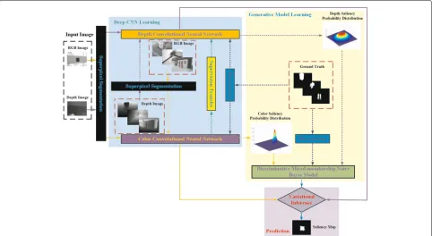
In this section, we introduce a method that integrates the colour saliency probability with the depth saliency probability computed from Gaussian distributions based on deep features and yields a prediction of the final 3D saliency map using the DMNB model within a Bayesian framework. The general architecture of the proposed framework is presented in Fig. 1.

First, we train a CNN model for depth images by teach-ing the network to reproduce the mid-level semantic rep-resentation learned from RGB images for which there are paired images. Then, deep features of the RGB and depth images are extracted by a CNN.

Second, the class-conditional mutual information (CMI) is computed to measure the dependence of the deep features of the RGB and depth images; then, the posterior probability of the RGB-D saliency is formulated by applying Bayes’ theorem. These two features com-plement each other in detecting 3D saliency cues from different perspectives and, when combined, yield the final 3D saliency value. By assuming that deep features are Gaussian distributions, the parameters of the Gaussian

distribution can be estimated in the DMNB model using a variational inference-based expectation maximization (EM) algorithm.

3.1 Feature extraction using CNN

Most existing saliency detection methods focus on how to design low-level saliency cues or model background priors. Low-level saliency cues alone do not produce good saliency detection results, particularly when salient objects are present in a low-contrast background with confusing visual cues. Objects cannot be classified as salient objects from the low-contrast background either based on low-level saliency cues or background priors, but they are semantically salient in high-level cognition as they are distinct in object categories. Due to its capa-bility of learning high-level semantic features, a CNN is effective for estimating the saliency maps of images and has been used for saliency detection [27, 28]. A CNN is able to generate representative and discriminative hyper-features rather than hand-designing heuristical hyper-features for saliency.

To better detect semantically salient objects, it is impor-tant to use high-level knowledge on object categories.

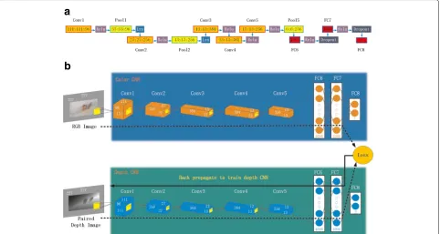
We employ deep convolutional neural networks to model the saliency of objects in RGB images and depth images. As shown in Fig. 2, the upper branch of our saliency detection pipeline is a deep CNN architecture with global context for RGB images, and the lower branch of our saliency detection pipeline is a deep CNN architecture with global context for depth images. For RGB images, the Clarifai [29] model is adopted as the baseline model, and a task-specific pre-training scheme is designed to make the global-context modelling suitable for saliency detec-tion [27]. We use a CNN similar to the Clarifai model for saliency detection with a pre-training using supervision transfer [30] for limited labelled depth images. The super-vision transfer occurs at the penultimate layer of the global context model. Taking the output of the penultimate layer of the two global context models as input, the DMNB model is trained to classify background and saliency, indi-cating the probabilities of whether a centred superpixel is in the background or belongs to a salient object.

3.1.1 Deep features of RGB image

Superpixel segmentation is first performed on RGB-D images [31], and the input of the global-context CNN is

a

b

a superpixel-centred large context window that includes the full RGB image. Regions that exceed the image bound-aries are padded with the mean pixel value of the RGB training dataset. The padded images are then warped to 227×3 as input, where the three dimensions represent width, height, and number of channels. With this normal-ization and padding scheme, the superpixel to be classified is always located at the centre of the RGB image, and the spatial distribution of the global context is normalized in this way. Moreover, it ensures that the input covers the entire range of the original RGB image. We refer readers to [27] for further details.

3.1.2 Deep features of depth image

We demonstrate how we transfer supervision from RGB images to depth images as obtained from a range sen-sors, such as the Microsoft Kinect, for the downstream task of saliency detection. We consider the domain of RGB images as Ms for which there is large dataset of

labelled images Ds, and we treat depth images as Md

with limited labelled dataD_dfor which we would like to train a rich representation for saliency detection. We use convolutional neural networks as our layered rich repre-sentation. For our layered image representation models, we use CNNs with the network architecture from the Clarifai model.

We denote the deep features of the RGB image as a corresponding K layered rich representation =

{φi

Ms,Ds,∀i ∈[1· · ·K]}. φ

i

Ms,Ds is the i

th _{layer of the}

Clarifai model for modalityMsthat has been trained on

labelled images from datasetDs. Now, we want to learn

the deep features of depth images from modalityMd, for

which we do not have access to a large dataset of labelled depth images. We have already hand-designed an appro-priate CNN architecture = {ψ_Mi

d,∀i ∈[ 1· · ·L]}from the Clarifai model. The task is then to effectively learn the parameters associated with various operations in the CNN architecture without having access to a large set of annotated images for modalityMd.

The scheme for training the depth CNN for depth images of modalityMdis to learn the parameters of CNN such that feature vectors from ψ_DL

d(Id) for image Id match the feature vectors from ψ_Mi∗_s,Ds(Is) for its image

pairIs in modality Ms for some chosen and fixed layer

i∗ ∈[1· · ·K]. By paired images, we mean a set of images of the same scene in two different modalities. We denote these parameters of CNNW_d[1···L] = {w_di,∀i ∈[1· · ·L]} to be learned by supervision transfer from layeri∗inof modalityMsto layerLinof modalityMd:

min

W_d[1···L]

(Is,Id)∈Us,d

f(ψ_ML _d(Id),φi

∗

Ms,Ds(Is)) (1) where Us,d denotes the NLPR dataset, which includes

paired images from modalitiesMsandMd. For the loss

functionf, we use theL2distance between the feature

vec-tors,f(·)= || · ||2₂. Then, the deep features of depth images are extracted by CNN.

3.2 Bayesian framework for saliency detection

Let the binary random variablezsdenote whether a point

belongs to a salient class. Given the observed deep fea-tures of RGB image xc and the deep features of depth

imagexdof that point, we formulate the saliency detection

as a Bayesian inference problem to estimate the posterior probability at each pixel of the RGB-D image:

p(zs|xc,xd)=

p(zs,xc,xd)

p(xc,xd)

(2)

wherep(zs|xc,xd)is shorthand for the probability of

pre-dicting whether a pixel is salient, p(xc,xd) is the

like-lihood of the observed deep features of RGB images and depth images, andp(zs,xc,xd) is the joint

probabil-ity of the latent class and observed features, defined as

p(zs,xc,xd)=p(zs)p(xc,xd|zs).

In this paper, the class-conditional mutual informa-tion (CMI) is used as a measure of the dependence between two featuresxcandxd, which can be defined as

I(xc,xd|zs) = H(xc|zs)+H(xd|zs)−H(xc,xd|zs), where

H(xc|zs) is the class-conditional entropy of xc, defined

as −_ip(zs = i)xcp(xc|zs = i)logp(xc|zs = i). Mutual information is zero whenxcandxdare mutually

independent given classzsand increases with increasing

level of dependence, reaching the maximum when one feature is a deterministic function of the other. Indeed, the independence assumption becomes more accurate with decreasing entropy, which yields an asymptotically optimal performance of the naive Bayes classifier [32].

The visual result for class-conditional mutual informa-tion between the deep features of RGB images and depth images on the NLPR dataset is shown in Fig. 5. We employ a CMI thresholdτ to discover feature dependen-cies. For CMI between the deep features of RGB images and depth images less thanτ, we assume thatxcandxd

are conditionally independent given the classeszs, that is,

p(xc,xd|zs) = p(xc|zs)p(xd|zs). This entails the

assump-tion that the distribuassump-tion of the deep features of RGB images does not change with the deep features of depth images. Thus, the pixel-wise saliency of the likelihood is given byp(zs|xc,xd)∝p(zs)p(xc|zs)p(xd|zs).

3.3 Generative model for saliency estimation

Given the graphical model of DMNB for saliency detec-tion shown in Fig. 3, the generative process for {x1:N,y}

Fig. 3Graphical models of DMNB for saliency estimation.yandxare the corresponding observed states, andzis the hidden variable, where each featurexjis assumed to have been generated from one

ofCGaussian distributions with a mean of_{μjk, [j]N1}and a variance of {σ2

jk, [j]N1}, andyis either 0 or 1, indicating whether the pixel is salient

Algorithm 1 Generative process for saliency detection following the DMNB model

1: Input:C.

2: Initialization:α,η.

3: Choose a component proportion:θ ∼Dir(θ|α). 4: For each feature:

choose a componentzj∼Mult(zj|θ);

choose a feature valuexj∼p(xj|zj,j).

5: Choose the label:y∼p(y|zj,η).

the number of features, andyis the label that indicates whether the pixel is salient.

In this work, the deep features of both RGB and depth images are assumed to have been generated from a Gaussian distribution with a mean of {μjk, [j]N1 }

and a variance of {σ_jk2, [j]N₁ }. The marginal distribution of(x1:N,y)is

p(x1:N,y|α,,η)=

p(θ|α)

⎛ ⎝N

j=1

zj

p(zj|θ)p(xj|zj,j)p(y|zj,η) ⎞ ⎠dθ

(3)

whereθis the prior distribution overCcomponents,=

{(μjk,σjk2), [j]N1 , [k]C1}are the parameters for the

distribu-tions of N features, andp(xj|zj,j) N(xj|μjk,σjk2). In

two-class classification,yis either 0 or 1 generated from

Bern(y|η). Because the DMNB model assumes a genera-tive process for both the labels and features, we use both X = {(xij), [i]M1 , [j]N1 }andY= {yi, [i]M1 }as a collection

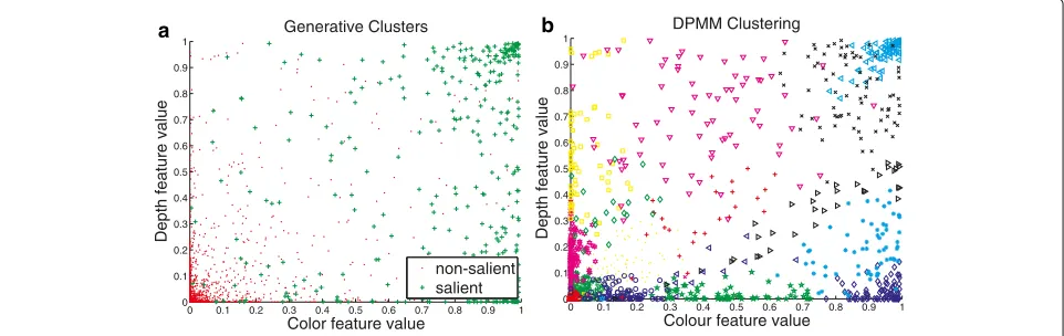
ofMsuperpixels in trained images from the generative process to estimate the parameters of the DMNB model such that the likelihood of observing(X,Y)is maximized. In practice, we may find a proper C using the Dirichlet process mixture model (DPMM)[33]. The DPMM thus provides a nonparametric prior for the parameters of a mixture model that allows the number of mixture compo-nents to increase as the training set increases, as shown in Fig. 6.

Due to the latent variables, the computation of the likelihood in Eq. 3 is intractable. In this paper, we use a variational inference method, which alternates between obtaining a tractable lower bound to the true log-likelihood and choosing the model parameters to maximize the lower bound. By directly applying Jensen’s inequality [14], the lower bound to logp(y,x1:N|α,,η)is

given by

logp(y,x1:N|α,,η)≥Eq(logp(y,x1:N,z1:N|α,,η))

+H(q(z1:N,θ|γ,φ)) (4)

Noting that x1:N and y are conditionally independent

givenz1:N, we use a variational distribution:

q(z1:N,θ|γ,φ)=q(θ|γ ) N

j=1

q(zj|φ) (5)

whereq(θ,γ )is aC-dimensional Dirichlet distribution for

θ andq(zj|φ)is a discrete distribution forzj. We useLto

denote the lower bound:

L=Eq[ logp(θ|α)]+Eq[ logp(z1:N|θ)]

+Eq[ logp(x1:N|z1:N,γ )]

−Eq[logq(θ)]−Eq[logq(z1:N)]+Eq[logp(y|z1:N,η)]

(6)

where Eq[ logp(y|z1:N,η)]≥

_C

k=1φk(ηky − e

ηk ξ ) −

(1

ξ + logξ) and ξ > 0 is a newly introduced

varia-tional parameter. Maximizing the lower-bound function L(γk,φk,ξ;α,,η)with respect to the variational

param-eters yields updated equations forγk,φkandξas follows:

φk ∝e

((γk)−(

C

l=1γl)+N1(ηkyi−e ηk

ξ −Nj=1 (xij−μjk)2

2σ2 jk

)) (7)

γk =α+Nφk (8)

ξ =1+C

k=1φke

ηk ₍₉₎

The variational parameters(γ∗,φ∗,ξ∗)from the infer-ence step provide the optimal lower bound to the log-likelihood of(xi,yi), and maximizing the aggregate lower

boundM_i=1L(γ∗,φ∗,ξ∗,α,,η)over all data points with respect to α, andη, respectively, yields the estimated

parameters. For μ, σ andη, we have μjk =

_M

i=1φikxij

_M

i=1φik ,

σjk =

_M

i=1φik(xij−μjk)2

_M

i=1φik

, andη_k=log(

_M

i=1φikyi

_M

i=1 φik

ξi

).

Algorithm 2Variational EM algorithm for DMNB 1: Input:thresholdε_L.

2: repeat

3: E-step:Given(α(t−1),(t−1),η(t−1)), for each feature value and label, find the optimal variational parame-ters using (10).

Then, L(γ_i(t),φ(_it),ξ_i(t);α,,η) provides a lower bound to logp(y_i,xi|α,,η).

4: M-step:Improved estimate of the model parameters

(α,,η) are obtained by maximizing the aggregate lower bound (11).

5: untilL(γ_i(t),φ_i(t),ξ_i(t);α(t),(t),η(t))

−L(γ(t+1)

i ,φ

(t+1)

i ,ξ

(t+1)

i ;α(t+1),(t+1),η(t+1)) ≤

εL

an initial guess(α0,0,η0), the variational EM algorithm alternates between two steps, as follows (Algorithm 2).

γ(t)

i ,φ(

t)

i ,ξ(

t)

i

=arg max γi,φi,ξi

Lγi,φi,ξi;α(t−1),(t−1),η(t−1)

(10)

α(t)_,(t)_,η(t)_{=arg max}

(α,,η) M

i=1

Lγ(t)

i ,φ(

t)

i ,ξ(

t)

i ;α,,η

(11)

After obtaining the DMNB model parameters from the EM algorithm, we can useηto perform saliency predic-tion. Given the featurex1:N, we have

E[ logp(y|x1:N,α,,η)]=

ηT_{E[z]−E[ log(1+e}ηTz_{)] y=1}

0−E[ log(1+eηTz_{)] y=0}

(12)

where z is an average of z1:N over all of the observed

features. The computation forE[z] is intractable; there-fore, we again introduce the distribution q(z1:N,θ) and

calculateEq[z] as an approximation ofE[z]. In

particu-lar,Eq[z]= φ; therefore, we only need to compare ηTφ

with 0.

3.4 Experimental evaluation

3.5 Generative model for saliency estimation

3.5.1 Evaluation datasets

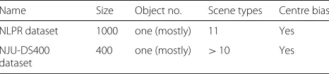
In this section, we conduct some experiments to demon-strate the performance of our method. We use the NLPR dataset1and NJU-DS400 dataset2to evaluate the perfor-mance of the proposed model, as shown in Table 1. The NLPR dataset [19] includes 1000 images of diverse scenes in real 3D environments, where the ground-truth was obtained by requiring five participants to select regions where objects are present, i.e. the salient regions were marked by hand. The NJU-DS400 dataset [10] includes

Table 1Comparison of the benchmark and existing 3D saliency detection datasets

Name Size Object no. Scene types Centre bias

NLPR dataset 1000 one (mostly) 11 Yes

NJU-DS400 dataset

400 one (mostly) >10 Yes

400 images of different scenes, where the ground-truth was obtained by four volunteers labelling the salient object masks.

We will analyse the 3D saliency situation in RGB-D images based on human judgement. In terms of the NLPR dataset [19], the 3D saliency is decided jointly by RGB images and depth images, as shown in Fig. 4. For each selected image pair from NLPR dataset, three participants are asked to draw a rectangle according to their first glance at the the most attention-grabbing region in RGB image and depth image, respectively. The 3D saliency situation is determined by thresholding the overlap ratio between the rectangle and the corresponding ground truth salient object mask. We use the Intersection over Union (IOU) to measure the match between bounding boxes and the ground truth, respectively. The IOU threshold is set at 0.5. The 3D saliency situation in RGB-D images follows three conditions:

Colour-depth saliency, in which both IOU values of RGB images and depth images are more than the IOU threshold, defined asDb = {I_cb,I_db}, where I_cb andI_db denote RGB images and depth images, respectively.

Colour saliency, in which only IOU values of RGB images are more than the IOU threshold and IOU values of depth images are less than the IOU threshold, defined asDc= {I_cc,I_dc}, whereI_ccandI_dcdenote RGB images and depth images, respectively.

Depth saliency, in which only IOU values of depth images are more than the IOU threshold and IOU values of RGB images are less than the IOU threshold, defined as Dd_=Id

c,Idd

, whereId

c andIdddenote RGB images and

depth images, respectively.

Fig. 43D saliency situation in RGB-D images.aColour-depth saliency: both RGB images and depth images are salient.bColour saliency: only RGB images are salient.cDepth saliency: only depth images are salient

3.5.2 Evaluation metrics

There are currently no specific and standardized mea-sures for computing the similarity between the fixation density maps and saliency maps created using computa-tional models in 3D situations. Nevertheless, there is a range of different measures that are widely used to per-form comparisons of saliency maps for 2D content. We introduce two types of measures to evaluate algorithm performance on the benchmark. The first one is the gold standard: F-measure. The second is the precision-recall (PR) curve. A continuous saliency map can be converted into a binary mask using a threshold, resulting in a pair of precision and recall values when the binary mask is compared against the ground truth. A PR curve is then obtained by varying the threshold from 0 to 1. The PR curve indicates the mean precision and recall of the saliency map at various thresholds.

3.5.3 Implementation details

We follow the default setup of the MC procedure from [27] for training the depth CNN using the caffe CNN library [34]. For training the depth CNN using supervision transfer, we copy the weights from the RGB CNN [27] that was pre-trained on ImageNet Large-Scale Visual Recog-nition Challenge (ILSVRC) 2014 [35] and fine-tuned for saliency detection on the MSRA10K dataset [36] to initial-ize this network, base the learning rate at 0.001 and step it down by a factor of 10 every 1000 iterations, except that we fine-tune all the layers. We randomly select 600 depth images I_db for training and 100 for validation fromDb. From each depth image, we select an average 200 of super-pixels, and in total, approximately 120 thousand input windows for training and 20 thousand for validation are

Table 23D saliency situation in terms of the NLPR dataset

Dataset Colour-depth saliency Colour saliency Depth saliency

NLPR 76.7% 20.8% 2.5%

generated. We label a patch as salient if 50% of the pix-els in this patch are salient; otherwise, it is labelled as non-salient. Training of the depth CNN for 10 thousand iterations costs 60 h without a GPU.

3.5.4 Parameter settings

A summary of the parameters in this paper is shown in Table 3. To evaluate the quality of the proposed approach, we divided the datasets into two subsets according to their CMI values, and we kept 20% of the data for testing purposes and trained on the remaining 80% whose CMI values are less than the CMI threshold τ. As shown in Fig. 5, we compute the CMI for all of the RGB-D images, and the parameterτ is set to 0.2, which is a heuristically determined value.

We initialize the model parameters using all data points and their labels in the training set in Algorithm 1. In par-ticular, we use the mean and standard deviation of the data points in each class to initialize and the ratio of data points in different classes to initializeαi.

3.5.5 The effect of the parameters

The parameter Cin Algorithm 1 is set according to the training set based on DPMM, as shown in Fig. 6. The appropriate number of mixture components to use in the DMNB model for saliency estimation is generally unknown, and DPMM provides an attractive alternative

Table 3The parameters and their settings in this paper

Name Range Description

τ (0,1) A CMI threshold

α (0, 40] The parameter of a Dirichlet distribution

θ (0,1) The parameter of a multinomial distribution

η (−2.0,2.0) The parameter of a Bernoulli distribution

((0,1),(0,0.2)) The parameter of a Gaussian distribution

a

b

c

Fig. 5Visual result for class-conditional mutual information between deep features of RGB images and depth images on the NLPR dataset, where blue star denotes the CMI value and red rectangle denotes the CMI histogram. The 3D saliency situation in RGB-D images is defined as colour-depth saliency, colour saliency, and depth saliency.aColour-depth saliency.bColour saliency.cDepth saliency

to current methods. In practice, we find the initial number of componentsCusing the DPMM based on 90% of the training set, and then we perform a cross validation with a range ofCby holding out 10% of the training data as the validation data.

We use 10-fold cross-validation with the parameterC

for DMNB models. In a 10-fold cross-validation, we divide the dataset evenly into 10 parts, one of which is selected as the validation set, and the remaining 9 parts are used as the training set. The process is repeated 10 times, with each part used once as the validation set. We use perplex-ity as the measurement for comparison. The generative models are capable of assigning a log-likelihood logp(xi)

to each observed data pointxi. Based on the log-likelihood

scores, we compute the perplexity of the entire dataset as perplexity = exp−M_i=1logp(xi)

M

, whereM is the number of data points. The perplexity is a monotonically decreasing function of the log-likelihood, implying that a lower perplexity is better (particularly on the test set)

since the model can explain the data better. We calculate the perplexity for results on the validation set and train-ing set, as shown in Fig. 7. Finally, for all the experiments described below, the parameterCwas fixed at 24, and no user fine-tuning was performed.

3.5.6 Compared methods

Let us compare our saliency model (BFSD) with a number of existing state-of-the-art methods, including graph-based manifold ranking (GMR)[7]; multi-context deep learning (MC)[27]; multiscale deep CNN (MDF)[28]; anisotropic centre-surround difference (ACSD)[10]; saliency detection at low-level, mid-level, and high-level stages (LMH)[19]; and exploiting global priors (GP)[20], among which GMR, MC and MDF are developed for RGB images, LMH and GP for RGB-D images, and ACSD for depth images. All of the results are produced using the public codes that are offered by the authors of the previously mentioned literature reports.

0 0.1 0.2 0.3 0.4 0.5 0.6 0.7 0.8 0.9 1 0

0.1 0.2 0.3 0.4 0.5 0.6 0.7 0.8 0.9 1

Generative Clusters

Color feature value

Depth feature value

non-salient salient

0 0.1 0.2 0.3 0.4 0.5 0.6 0.7 0.8 0.9 1 0

0.1 0.2 0.3 0.4 0.5 0.6 0.7 0.8 0.9 1

DPMM Clustering

Colour feature value

Depth feature value

a b

-1.1 -1 -0.9 -0.8 -0.7 -0.6 -0.5 -0.4 -0.3 -0.2

Perplexity

C=12 C=16 C=20 C=24 C=28 C=32 C=36

train test train test train test train test train test train test train test

Fig. 7Cross validation. We use 10-fold cross-validation with the parameterCfor DMNB models. TheCfound using DPMM was adjusted over a wide range in a 10-fold cross-validation

3.6 Qualitative experiment

3.6.1 Colour-depth saliency

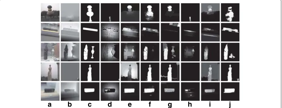
In this case, both RGB images and depth images are salient. The comparison of the state-of-the-art approaches is presented in Fig. 8. As shown in the first and seventh

rows of Fig. 8, the salient object has a high colour contrast with the background; thus, RGB saliency methods are able to correctly detect salient objects. GMR fails to detect many pixels on the prominent objects because it does not define the pseudo-background accurately, e.g. the third

a

b

c

d

e

f

g

h

i

j

row in Fig. 8. As shown, the proposed method can accu-rately locate the salient objects and produce nearly equal saliency values for the pixels within the target objects.

3.6.2 Colour saliency

In this case, only RGB images are salient. The comparison of the state-of-the-art approaches is presented in Fig. 9. ACSD works on depth images on the assumption that salient objects tend to stand out from the surrounding background, which takes relative depth into considera-tion. ACSD performs worse when the salient object lies in the same plane as the background, e.g. the third row in Fig. 9. It is challenging because most of the salient objects share similar depth as the background. Conse-quently, depth saliency methods perform relatively worse than RGB saliency methods in terms of precision. Ren et al. proposed two priors, which are the normalized depth prior and the global-context surface orientation prior [20]. Because their approach uses the two priors, it has prob-lems when such priors are invalid, e.g. the first row in Fig. 9. Figure 9 shows that the proposed method consis-tently outperforms all the other saliency methods.

3.6.3 Depth saliency

In this case, only depth images are salient. The compar-ison of the state-of-the-art approaches is presented in Fig. 10. When a salient object shares a similar colour with the background, it is difficult for existing RGB models to extract saliency. With the help of depth information, a salient object can easily be detected by the proposed RGB-D method. In particular, when the salient object shares similar object categories, e.g. the first row in Fig. 10, MC and MDF generate unsatisfying results without depth cues. ACSD is not designed for such complex scenes but

rather single dominant-object depth images. By providing an accurate depth map, the LMH and GP methods per-form well in both precision and recall. LMH uses a simple fusion framework that takes advantage of both depth and appearance cues from the low, mid, and high levels. The background is nicely excluded; however, many pixels on the salient object are not detected as salient, e.g. the sec-ond row in Fig. 10. Figure 10 also shows that the proposed method consistently outperforms all the other saliency methods.

3.7 Quantitative evaluation

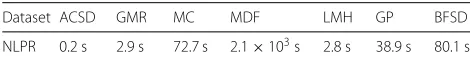
Our algorithm is implemented in MATLAB v7.12 and tested on an Intel Core(TM) i5-6400 CPU with 8 GB of RAM. A simple computational comparison is shown in Table 4 in terms of the NLPR dataset without a GPU. The run time of ACSD is for per depth image; GMR, MC and MDF are for per RGB image; and LMH, GP and BFSD are for per RGB-D image pair. Note that there are many works left for computational optimization, including optimiza-tion of prior parameters and algorithm optimizaoptimiza-tion for variable inference during the prediction process.

The quantitative comparisons on the NLPR dataset are shown in Figs. 11 and 12. As shown in Fig. 11a, b, although the PR curves are very similar in the colour-depth saliency situation and the colour saliency situation, Fig. 11c shows that the proposed method is superior com-pared to MC and MDF in the depth saliency situation. The LMH method, which uses Bayesian fusion to fuse depth and RGB saliency by simple multiplication, has lower per-formance compared to the GP method, which uses the Markov random field model as a fusion strategy, as shown in Fig. 11b, c. LMH and GP achieve better performances than ACSD by using fusion strategies, as shown in Fig. 11.

a

b

c

d

e

f

g

h

i

j

Fig. 9Visual comparison of the saliency detection in the colour saliency situation in terms of the NLPR dataset.aRGB.bDepth.cGround truth.d

a

b

c

d

e

f

g

h

i

j

Fig. 10Visual comparison of the saliency detection in the depth saliency situation in terms of the NLPR dataset.aRGB.bDepth.cGround truth.d

ACSD.eGMR.fMC.gMDF.hLMH.iGP.jBFSD

LMH and GP achieve better performances than GMR by using fusion strategies in the depth saliency situation, as shown in Fig. 11c; however, LMH and GP achieve lower performances in the colour saliency situation, as shown in Fig. 11b. The PR curves demonstrate that the proposed 3D saliency detection model performs better than do the compared methods overall, as shown in Fig. 11d. We also provide the F-measure values for several compared meth-ods in Table 5, which shows that the proposed RGB-D method is superior to the existing methods in terms of F-measure values. This result is mainly because the deep features of RGB-D images extracted by CNNs enhance the consistency and compactness of salient patches.

As shown in Fig. 12c, in the depth saliency situa-tion, the RGB saliency methods perform relatively worse than the RGB-D saliency methods in terms of precision. However, in the colour saliency situation, the ACSD and LMH methods do not perform well in both precision and recall. Although the simple late fusion strategy achieves improvements in the depth saliency situation, as shown in Fig. 12c, it still suffers from inconsistency in the homoge-neous foreground regions in the colour saliency situation, as shown in Fig. 12b, which may be attributed to treat-ing the appearance and depth correspondence cues in an independent manner. In the colour-depth saliency situa-tion, due to the capability of learning high-level semantic features, MC and MDF perform relatively better than the LMH and GP methods in terms of F-measure. Although the recall values are very similar, Fig. 12b, c show that the proposed method improves the precision and F-measure when compared to MC and MDF. Our approach consis-tently detects the pixels on the dominant objects within a Bayesian framework with higher accuracy to resolve the

Table 4Comparison of the average run time (seconds) on the NLPR dataset

Dataset ACSD GMR MC MDF LMH GP BFSD

NLPR 0.2 s 2.9 s 72.7 s 2.1×103_{s 2.8 s 38.9 s 80.1 s}

issue. Figure 12 shows that the proposed method performs favourably against the existing algorithm with higher pre-cision, recall values, and F-measure scores on the NLPR dataset.

3.7.1 Supervision transfer vs fine-tuning

This section investigates the effectiveness of different depth CNN learning strategies. It was demonstrated that fine-tuning a deep CNN model for image classification with the target task (e.g. object detection) data can signif-icantly improve the performance of the target task [37]. Supervision transfer enables learning of rich representa-tions from a large labelled modality as a supervisory signal for training representations for a new unlabelled paired modality and can be used as a pre-training procedure for new modalities with limited labelled data. However, the fine-tuning task and the supervision transfer task have disparity in the following aspects. (1) Input data. The fine-tuning task takes the labelled depth images as inputs, while the supervision transfer task requires the paired RGB and depth images. The fine-tuning solve the problem of domain adaptation within the same modality. In contrast, supervision transfer here tackles the prob-lem of domain adaptation across different modalities. (2) The adapted layer. The fine-tuning task adapts the last soft-max layer to the same modality data, while the super-vision transfer happens at the arbitrary internal layer for a new image modality. Particularly, deep model struc-tures at the fine-tuning stage are only different in the last fully connected layer for predicting labels. Supervision transfer here allows for transfer of supervision at arbi-trary semantic levels. Due to the “data-hungry” nature of CNNs, the existing training data is insufficient for train-ing; therefore, we employed supervision transfer to resolve this issue.

0.5 1.0 0.5 1.0 Recall Precision PR curve ACSD GMR MC MDF LMH GP BFSD 0.5 1.0 0.5 1.0 Recall Precision P-R curve ACSD GMR MC MDF LMH GP BFSD 0.5 1.0 0.5 1.0 Recall Precision PR curve ACSD GMR MC MDF LMH GP BFSD 0.5 1.0 0.5 1.0 Recall Precision PR curve ACSD GMR MC MDF LMH GP BFSD

a

b

c

d

Fig. 11The PR curves of different saliency detection models in terms of the NLPR dataset.aColour-depth saliency.bColour saliency.cDepth saliency.dThe overall

compared with fine-tuning with depth images, as shown in Fig. 13. We use the Clarifai that has been trained on labelled images in the ImageNet dataset, and use the mid-level representation learned by the CNN as a supervisory signal to train a CNN on depth images. Note that the out-put of the penultimate layer of Depth CNN is indeed a feature vector for saliency detection. The technique for transferring supervision results in improvements in per-formance for the end task of saliency detection on NLPR dataset, where we improve from 1.5 to 1.9% when using both RGB and depth images together, compared with the fine-tuning when using just the depth images. From the results on NLPR dataset in Fig. 13, we can conclude that supervision transfer outperforms the conventional fine-tuning method, which validates the effectiveness of the proposed supervision transfer approach for saliency detection.

3.7.2 Fusion strategy comparison

Despite the demonstrated success of deep features extracted from RGB images and Depth images, no single feature is effective for all scenarios as they define saliency from different perspectives. The combination of differ-ent features might be a good solution to visual saliency detection for RGB-D images. However, manually design-ing an interaction mechanism for integratdesign-ing inherently different saliency features is a challenging problem. The

qualitative comparisons and quantitative comparisons of the different fusion strategies using the deep CNN fea-tures are shown in Figs. 14, 15, and 16, respectively. CSM means colour saliency map, which is produced by deep features of the colour CNN. DSM means depth saliency map, which is produced by deep features of the depth CNN. We add and multiple the CSM with the DSM, and these results are denoted CSM+CSM and CSM×DSM. As shown in Fig. 14, neither simple lin-ear fusion nor weighting method is subsequently able to recover the salient object. Both simple linear fusion and weighting method suffer from inconsistency in the homo-geneous foreground regions and lacks precision around object boundaries, which may be ascribed to treating the colour and depth correspondence cues in an indepen-dent manner. Our approach consistently detects the pixels on the dominant objects within a Bayesian framework with higher accuracy to resolve the issue. Figure 15 shows that the Bayesian fusion performs favourably compared with the linear fusion and the weighting method, with higher precision and recall on the NLPR dataset. Although the simple late fusion strategy achieves improvements, it still suffers from inconsistency due to ignore the strong complementarities between appearance and depth correspondence cues. We adopt a good integration method developed to address this problem by training a generative model.

ACSD GMR MC MDF LMH GP BFSD 0 0.1 0.2 0.3 0.4 0.5 0.6 0.7 0.8 Recall Precison F-Measure

ACSD GMR MC MDF LMH GP BFSD 0 0.1 0.2 0.3 0.4 0.5 0.6 0.7 0.8 Recall Precison F-Measure

ACSD GMR MC MDF LMH GP BFSD 0 0.1 0.2 0.3 0.4 0.5 0.6 0.7 0.8 0.9 1 Recall Precison F-Measure

ACSD GMR MC MDF LMH GP BFSD 0 0.1 0.2 0.3 0.4 0.5 0.6 0.7 0.8 0.9 Recall Precison F-Measure

a

b

c

d

Table 5Comparison of the F-measure on the NLPR dataset

3D saliency situation ACSD GMR MC MDF LMH GP BFSD

Colour-depth saliency 0.5548 0.6540 0.7381 0.6983 0.6109 0.6891 0.7793

Colour saliency 0.5195 0.6612 0.6684 0.6630 0.5645 0.6480 0.7658

Depth saliency 0.5635 0.7032 0.7711 0.7689 0.7744 0.8095 0.9044

Overall 0.5510 0.6652 0.7366 0.7058 0.6317 0.7082 0.8092

The best results are shown in Italics

2K 6K 10K 14K 18K

0.695 0.7 0.705 0.71

F-measure score

Iterations

Supervision transfer Fine-tuning

a

b

c

d

e

f

Fig. 13Evaluation of the depth CNN learned using different training strategies on the NLPR dataset.aF-measure scores on the NLPR dataset for evaluation of the supervision transfer (ST) strategy and the fine-tuning (FT) strategy.b–fQualitative comparison between the ST strategy and the FT strategy for 10k iterations

a

b

c

d

e

f

g

h

Fig. 14Visual comparison of different fusion strategies in terms of the NLPR dataset.aRGB.bDepth.cGround truth.dCSM.eDSM.fCSM+DSM.g

0.5 1.0 0.5 1.0 Recall Precision PR curve CSM DSM CSM + DSM CSM X DSM BFSD 0.5 1.0 0.5 1.0 Recall Precision PR curve CSM DSM CSM + DSM CSM X DSM BFSD 0.5 1.0 0.5 1.0 Recall Precision PR curve CSM DSM CSM + DSM CSM X DSM BFSD 0.5 1.0 0.5 1.0 Recall Precision PR curve CSM DSM CSM + DSM CSM X DSM BFSD

a

b

c

d

Fig. 15The PR curves of different fusion strategies in terms of the NLPR dataset.aColour-depth saliency.bColour saliency.cDepth saliency.dThe overall. The symbol “+” indicates a linear combination strategy, and the symbol “×” indicates a weighting method based on multiplication

3.8 Cross-dataset generalization

In this section, we evaluate the generalization perfor-mance of BFSD. To test how well the perforperfor-mance of our proposed method generalizes to a different dataset for detecting salient object in RGB-D images, we eval-uate it on the NJU-DS400[10]. As discussed in experi-ment setting, the images of the NJU-DS400 are collected in different scenarios. We directly test the performance on the NJU-DS400 dataset with the model learned on NLPR dataset. The results are shown in Figs. 17 and 18. In the NJU-DS400 dataset, we do not have experimen-tal results for the LMH and GP methods due to the lack of depth information, which is required by their codes. Although the model is trained on the NLPR dataset, it outperforms all other previous methods based on the F-measure scores and PR curves. This clearly demonstrates the generalization performance of our pro-posed method and robustness to dataset biases. Our model explores high-level information of RGB-D images to investigate semantics-driven attention to 3D content, and has much stronger generalization capability. Though Gaussian distributions of the DMNB model provide bet-ter performance than compared methods in bet-terms of NJU-DS400 dataset, different numbers of mixture com-ponent would impair the generalization capability of this

mixture model, especially in the case of multiple scene types.

3.8.1 Failure cases

Figure 19 presents more visual results and some failure cases of our proposed method on NLPR dataset. By com-paring these images, we find that semantic information is more helpful when the salient object shares a very sim-ilar colour and depth information with the background. Figure 20 presents additional visual results and a fail-ure case of our proposed method on NJU-DS400 dataset. We find that although our method is able to highlight the overall salient objects, the generated coarse maps may confuse some of small foreground or background regions if they have similar appearance. Our method may fail when the salient object shares a very similar colour and depth information with the background in a global context.

3.8.2 Limitations

Because our approach requires training on large datasets to adapt to specific environments, it has the problem that properly tuning the parameters for specific new tasks is important to the performance of the DMNB model. The DMNB model performs classification in one shot via a

CSM DSM CSM + DSMCSM x DSM BFSD 0 0.1 0.2 0.3 0.4 0.5 0.6 0.7 0.8 0.9 Recall Precison F-Measure

CSM DSM CSM + DSMCSM x DSM BFSD 0 0.1 0.2 0.3 0.4 0.5 0.6 0.7 0.8 0.9 Recall Precison F-Measure

CSM DSM CSM + DSMCSM x DSM BFSD 0 0.1 0.2 0.3 0.4 0.5 0.6 0.7 0.8 0.9 1 Recall Precison F-Measure

CSM DSM CSM + DSMCSM x DSM BFSD 0 0.1 0.2 0.3 0.4 0.5 0.6 0.7 0.8 0.9 Recall Precison F-Measure

a

b

c

d

Fig. 16The F-measure scores of different fusion strategies in terms of the NLPR dataset.aColour-depth saliency.bColour saliency.cDepth saliency.

a

b

c

d

e

f

g

h

Fig. 17Visual comparison of the saliency detection in terms of the NJU-DS400 dataset.aRGB.bDepth.cGround truth.dACSD.eGMR.fMC.g

ACSD GMR MC MDF BFSD 0

0.1 0.2 0.3 0.4 0.5 0.6 0.7 0.8

Recall Precison F-Measure

0.5 1.0

0.5 1.0

Recall

Precision

PR curve

ACSD GMR MC MDF BFSD

a

b

Fig. 18Experimental results on the NJU-DS400 dataset compared with previous works.aThe F-measure scores.bThe PR curves. F-measure scores and PR curves show superior generalization ability of a BFSD framework

combination of mixed-membership models and logistic regression, where the results may depend on different choices of C. The learned parameters will clearly have good performances on the specific stimuli but not nec-essarily on the new testing set. Thus, the weakness of the proposed method is that to obtain reasonable perfor-mances, we train our saliency model on the training set for specificC. This problem could be addressed by using Dirichlet process mixture models to find a properCfor new datasets.

4 Conclusion

In this study, we propose a learning-based 3D saliency detection model for RGB-D images that considers the deep features of RGB images and depth images within a Bayesian framework. To better detect semantically

salient objects, we employ a deep CNN to model saliency of objects in RGB images and depth images. Rather than simply combining a depth map with 2D saliency maps as in previous studies, we propose a compu-tational saliency detection model for RGB-D images based on the DMNB model. The experiments verify that the deep features of depth images can serve as a helpful complement to the deep features of RGB images within a Bayesian framework. Compared with other competing 3D models, the experimental results from a public RGB-D saliency datasets demonstrate the improved performance of the proposed model over other strategies.

As a future work, we are considering to improve the feature representation of the depth images. We are considering to represent the depth image by three

a

b

c

d

a

b

c

d

channels (horizontal disparity, height above ground, and angle with gravity) [38] for saliency detection because this representation allows the CNN to learn stronger features than by using disparity alone. We are also considering the application of our 3D saliency detec-tion model in RGB-D object detecdetec-tion problems, e.g. 3D object proposals.

Endnotes

1_{http://sites.google.com/site/rgbdsaliency}

2_{http://mcg.nju.edu.cn/en/resource.html}

Acknowledgements

This work was supported in part by the Beijing Municipal special financial project (PXM2016_278215_000013, ZLXM_2017C010) and by the Innovation Group Plan of Beijing Academy of Science and Technology (IG201506C2).

Authors’ contributions

SW took charge of the system coding, doing experiments, data analysis and writing the whole paper excluding variational EM algorithm part at subsection 3.3. ZZ took charge of advisor position for paper presentation and experiment design. WJ took charge of data analysis presentation as well as English revising. HQ took charge of coding and writing for variational EM algorithm part at subsection 3.3. All authors read and approved the final manuscript.

Competing interests

The authors declare that they have no competing interests.

Publisher’s Note

Springer Nature remains neutral with regard to jurisdictional claims in published maps and institutional affiliations.

Author details

1_{The Higher Educational Key Laboratory for Measuring and Control} Technology and Instrumentations of Heilongjiang Province, Harbin University of Science and Technology, Harbin, 150080 China.2_{Res. Center for Artif. Intell.} and Big Data Anal., Beijing Academy of Science and Technology, Beijing, 100094 China.

Received: 31 May 2017 Accepted: 13 December 2017

References

1. Le Callet P, Niebur E (2013) Visual attention and applications in multimedia technology. Proc IEEE 101(9):2058–2067. https://doi.org/10. 1109/JPROC.2013.2265801

2. Wang J, Fang Y, Narwaria M, Lin W, Callet PL (2014) Stereoscopic image retargeting based on 3d saliency detection. In: The IEEE International Conference on Acoustics, Speech and Signal Processing. IEEE, Florence. pp 669–673

3. Kim H, Lee S, Bovik C (2014) Saliency prediction on stereoscopic videos. IEEE Trans Image Process 23(4):1476–1490. https://doi.org/10.1109/TIP. 2014.2303640

4. Zhang Y, Jiang G, Yu M, Chen K (2010) Stereoscopic visual attention model for 3d video. In: The 16th International Conference on Multimedia Modeling. Springer, Chongqing. pp 314–324

5. Borji A, Cheng M, Hou Q, Jiang H, Li J (2017) Salient object detection: a survey. arXiv preprint arXiv:1411.5878

6. Borji A, Cheng M, Jiang H, Li J (2015) Salient object detection: a benchmark. IEEE Trans Image Process 24(12):5706–5722. https://doi.org/ 10.1109/TIP.2015.2487833

7. Yang C, Zhang L, Lu H, Ruan X, Yang M (2013) Saliency detection via graph based manifold ranking. In: The IEEE Conference on Computer Vision and Pattern Recognition. IEEE, Portland. pp 3166–3173 8. Peng H, Li B, Ling H, Hu W, Xiong W, Maybank SJ (2017) Salient object

9. Li B, Xiong W, Hu W (2012) Visual saliency map from tensor analysis. In: Proceedings of Twenty-Sixth AAAI Conference on Artificial Intelligence. AAAI, Toronto. pp 1585–1591

10. Ju R, Ge L, Geng W, Ren T, Wu G (2014) Depth saliency based on anisotropic centre-surround difference. In: IEEE International Conference Image Processing. IEEE, Pairs. pp 1115–1119

11. Song H, Liu Z, Xie Y, Wu L, Huang M (2016) Rgbd co-saliency detection via bagging-based clustering. IEEE Sig Process Lett 23(12):1722–1726. https://doi.org/10.1109/LSP.2016.2615293

12. Lang C, Ngugen T, Katti H, Yadati K, Kankanhalli M, Yan S (2012) Depth matters: influence of depth cues on visual saliency. In: The 12th European Conference Computer Vision. Springer, Florence. pp 101–105

13. Desingh K, Madhava K, Rajan D, Jawahar C (2013) Depth really matters: improving visual salient region detection with depth. In: The British Machine Vision Conference. BMVA, Bristol. pp 98.1–98.11 14. Shan H, Banerjee A, Oza N (2009) Discriminative mixed-membership

models. In: IEEE International Conference Data Mining. IEEE, Miami. pp 466–475

15. Fang Y, Wang J, Narwaria M, Le Callet P, Lin W (2014) Saliency detection for stereoscopic images. IEEE Trans Image Process 23(6):2625–2636. https://doi.org/10.1109/TIP.2014.2305100

16. Wu P, Duan L, Kong L (2015) Rgb-d salient object detection via feature fusion and multi-scale enhancement. In: Chinese Conference Computer Vision. Springer, Xi’an. pp 359–368

17. Ciptadi A, Hermans T, Rehg J (2013) An in depth view of saliency. In: The British Machine Vision Conference. BMVA, Bristol. pp 9–13

18. Iatsun I, Larabi M, Fernandez-Maloigne C (2014) Using monocular depth cues for modeling stereoscopic 3D saliency. In: IEEE International Conference Acoustics, Speech and Signal Processing. IEEE, Florence. pp 589–593

19. Peng H, Li B, Hu W, Ji R (2014) Rgbd salient object detection: a benchmark and algorithms. In: The 13th European Conference Computer Vision. Springer, Zurich. pp 92–109

20. Ren J, Gong X, Yu L, Zhou W (2015) Exploiting global priors for rgb-d saliency detection. In: IEEE Conference Computer Vision and Pattern Recognition Workshops. IEEE, Boston. pp 25–32

21. Xue H, Gu Y, Li Y, Yang J (2015) Rgb-d saliency detection via mutual guided manifold ranking. In: IEEE International Conference Image Processing. IEEE, Quebec. pp 666–670

22. Wang J, DaSilva M, Le Callet P, Ricordel V (2013) Computational model of stereoscopic 3D visual saliency. IEEE Trans Image Process

22(6):2151–2165. https://doi.org/10.1109/TIP.2013.2246176 23. Fang Y, Lin W, Fang Z, Lei J, Le Callet P, Yuan F (2014) Learning visual

saliency for stereoscopic images. In: IEEE International Conference Multimedia and Expo Workshops. IEEE, Chengdu. pp 1–6

24. Zhu L, Cao Z, Fang Z, Xiao Y, Wu J, Deng H, Liu J (2015) Selective features for RGB-D saliency. In: Conference Chinese Automation Congress. IEEE, Wuhan. pp 512–517

25. Bertasius G, Park H, Shi J (2015) Exploiting egocentric object prior for 3d saliency detection. arXiv preprint arXiv:1511.02682

26. Qu L, He S, Zhang J, Tian J, Tang Y, Yang Q (2013) RGBD salient object detection via deep fusion. IEEE Trans Image Process 26(5):2274–2285. https://doi.org/10.1109/TIP.2017.2682981

27. Zhao R, Ouyang W, Li H, Wang X (2015) Saliency detection by multi-context deep learning. In: IEEE Conference Computer Vision and Pattern Recognition Workshops. IEEE, Boston. pp 1265–1274

28. Li G, Yu Y (2016) Visual saliency detection based on multiscale deep CNN features. arXiv preprint arXiv:1609.02077

29. Zeiler M, Fergus R (2014) Visualizing and understanding convolutional networks. In: The 13th European Conference Computer Vision. Springer, Zurich. pp 818–833

30. Gupta S, Hoffman J, Malik J (2015) Cross modal distillation for supervision transfer. arXiv preprint arXiv:1507.00448

31. Wang S, Zhou Z, Qu H, Li B (2016) Visual saliency detection for RGB-D images with generative model. In: The 13th Asian Conference on Computer Vision. Springer, Taipei. pp 20–35

32. Rish I (2001) An empirical study of the naive Bayes classifier. J Univ Comput Sci 3(22):41–46

33. Blei D, Jordan M (2006) Variational inference for dirichlet process mixtures. Bayesian Anal 1(1):121–143

34. Jia Y (2013) Caffe: An open source convolutional arichitecture for fast feature embedding. http://caffe.berkeleyvision.org/. Accessed 2013 35. Russakovsky O, Deng J, Su H, Krause J, Satheesh S, Ma S, Huang Z,

Karpathy A, Khosla A, Bernstein M, Berg AC, Li F (2014) Imagenet large scale visual recognition challenge. Int J Comput Vis 115(3):211–252 36. Cheng M, Mitra N, Huang X, Torr P, Hu S (2014) Global contrast based on

salient region detection. IEEE Trans Image Process 37(3):569–582. https:// doi.org/10.1109/TPAMI.2014.2345401

37. Girshick R, Donahue J, Darrell T, Malik J (2013) Rich feature hierarchies for accurate object detection and semantic segmentation. arXiv preprint arXiv:1311.2524