How much methodology ror explains the rain errors in caibarién, cuba

ISSN: 2319-6505

HOW MUCH METHODOLOGY ROR EXPLAINS THE RAIN ERRORS IN CAIBARIÉN, CUBA

Osés Rodríguez, Ricardo

, Burgos Alemán, Iosbel

, Osés Llanes, Claudia

, Otero Martin Meylin

, C.

Fimia Duarte, Rigoberto

_{and Cruz Camacho, Lisvette}

4_{Faculty of Health Care Technology, Santa Clara, Cuba}

A R T I C L E I N F O A B S T R A C T

The objective of this work is to determine how much information the methodology ROR can give when having a series whose selfcorrelograms are a white noise. It was used the variable of the monthly fallen rain in Caibarién, Cuba, in the period 1977-2014. By using modeling ROR, it has been obtained information for the future projection of data series of errors by modeling ARIMA, as this type of modeling opens an important and promising way for the series that behave as white noise, by giving new information for the series and its behavior. The model explains the 8.7 % of variance, with errors of 44.6 mm. The errors tendency is the increase around 0.004 mm, although it is not statistically significant, the errors depend on the errors 1 month behind. All the work was carried out with the help of the statistical package of Social Sciences (SPSS) Version 13.

INTRODUCTION

The information in a data series is important when projecting the future, but: what happens when the modeling series is a white noise?, therefore there is no information in previous steps allowing to model towards the future. This article deals about methodology ROR and how through its use, important information can be obtained to project the future behavior of the series.

The Methodology ROR (Regression Objective Regressive1) is carried out in several steps which are explained in this article; however it is necessary to detail them since the mathematical point of view.

In this methodology, it is done an adjustment of curves using the method of square minimums, which are explained as follows.

It is frequently necessary to represent by means of a functional relation data that have been given as a group of points X - Y. For instance, an experiment has been made and the points X–Y have been obtained in a graphic of Y against X. As these points are going to be used for computer calculus, several problems have to be faced:

1. There are experimental errors in Y values. It should be softened somehow the variations due to experimental errors.

2. The value of Y is wanted corresponding to some value of X which is found between two experimental values of X.

3. It would be desirable– in fact it can be the main purpose of the calculus– to transfer, that is to determine the value of Y corresponding to a value of X out of the range of experimental values of this variable.

All these considerations lead to the necessity of a functional relation between X and Y in equation form, and hopefully simple. The question is then to determine a curve to approximate data with enough precision. The first question is this: How to decide if a curve given is a good "adjustment" to data?

This discussion will be simpler if a new term is defined now:

The deviation in a given point is the difference between the value of experimental Y and the calculated value of Y beginning from a functional relation. The question to adjust a curve to data can be reformulated: What conditions can be put to deviations to reach an adequate curve?

A possibility that could be attractive is to ask for the deviations sums can be as small as possible. If a prime is used to identify the values2 of Y calculated beginnning from the wanted functional relation, this means to ask for:

N

Σ( Yi- Yi

׳ ) i=1

Available Online at http://journalijcar.org

International Journal

of Current Advanced

Research

Vol 4, Issue 2, pp 17-21, February 2015

Article History:

Received5th, January, 2015

Received in revised form15th, January, 2015 Accepted12th, February, 2015

Published online 28th, February, 2015

© Copy Right, Research Alert, 2015, Academic Journals. All rights reserved.

RESEARCH ARTICLE

ISSN: 2319 - 6475

Key words:

be a minimum, in which N is the number of data points, but the attractive of this possibility disappears when considering the simple case of adjusting a line at two points. This difficulty could be avoided by specifying absolute values, that is requiring to minimize.

N

Σ I Yi- Yi

׳ I i=1

But it cannot be derived to find a minimum value because the function absolute value has no derivate in its minimum. It can be thought to ask for the maximum error is a minimum, which is Chebyshev approximation, but this leads to an iterative process complicated to determine the functional relation. This leads to the criterion of the square minimums, in which is inquired a minimum value of:

N

Σ ( Yi- Yi

׳ )2 i=1

As it can be observed, this expression can be different to determine its minimum and leads to equations that are linear in many cases of practical interest, and from the beginning, are easy to solve. Finally, there are statistical considerations that suggest the square minimums are a good criterion, besides its computer facility.

Thus it is written the function of approximation for methodology ROR as follows:

Yi

׳

= c1*δ1(xi) + c2*δ2(xi) + c3 *NoC(xi).

Where:

0 if Xi = 2n

δ1(xi) = { n= 0,1…N

1 if Xi = 2n +1.

1 if Xi = 2n

δ2(xi) = { n= 0,1…N

0 if Xi = 2n +1.

NoC(xi) = xi , xi = 0,1,…, N.

The objective is to determine C1, C2 and C3, to minimize:

N S=Σ( Yi- Yi

׳ )2 i=1

N

S= Σ ( Yi- c1*δ1(xi) - c2*δ2(xi) - c3 *NoC(xi)2

i=1

It is known that to minimize S considered as function of C1 is equals to zero the partial derivate of S with respect to C1, the result is:

N

(∂S/∂c1)= (-2)Σ( Yi- c1* δ1(xi) - c2* δ2(xi) - c3 *NoC(xi ) =0.

Making equal to zero and readjusting, it is obtained:

N N N N c1* (Σ δ1(xi)) + c2* (Σ δ2(xi)) + c3 *(ΣNoC(xi)) =ΣYi.

i=1 i=1 i=1 i=1

0 N N N c1* ( )+ c2* ( ) + c3 *(Σ(xi )) =ΣYi.

N 0 i=1 i=1

Deriving S with respect to C2 and then with respect to C3 and making each one of the results equal to zero, they are obtained two more equations in the incognitos C1, C2, C3, the three simultaneous equations in these three incognitos are named normal equations to adjust an equation to the data group, then:

0 N N N c1* ( )+ c2* ( ) + c3 *(Σ(xi)) =ΣYi.

N 0 i=1 i=1

0 N N N c1* ( )+ c2* ( ) + c3 *(Σ(xi )) =ΣYi.

N 0 i=1 i=1

0 N N N c1* ( )+ c2* ( ) + c3 *(Σ(xi)) =ΣYi.

N 0 i=1 i=1

To find a "better" function for data; it is only needed to carry out the necessary sums and solve the system of three equations, this combination explains great quantity of variance of Yi, and then it is obtained:

Yi

׳

= c1*δ1(xi) + c2*δ2(xi) + c3 *NoC(xi).

There are errors left ei= (Yi- Yi

׳

), then it is calculated the cross correlation of eiwith Yi-n(xi) in the following formula:

Cov(ei, Yi-n(xi))

Corr(ei, Yi-n(xi)) = --- and the

maximum value is selected of this

[Var (ei)*Var (Yi-n(xi)]1/2

function that is the corresponding peak named t, it is calculated then the variable Yt and the system is resolved

again, this time with the variable Yt,

(∂ei/∂ci)= (∂S2/∂ci) =0 this time with the function:

S2=(Yi–c1*δ1(xi) - c2*δ2(xi) - c3 *NoC(xi)–c4*Yt(xi))2,

Then there is an error left e2which is croscorrelated with g

i-k(xi) as hexogen variable, the same done with eiobtaining a

new peak in t for the variable gi-k(xi), and is resolved again the

system (t can be of different order to the calculated for the function Yi-n(xi).

This time (∂ei/∂ci)= (∂S3/∂ci)=0 in such way

At the end it is obtained an error e4which should have media

zero and variance 1 and the process is stopped obtaining the highest quantity of variance as possible, in this approximation data of the same function are used Yi-n(xi) and hexogen data

of the function gi-k(xi).

This methodology has been used in the model for variable angiostrongilosis3, where the following model of function was obtained:

Where DS=δ1(xi) and DI =δ2(xi) NoC= NoC(xi), is

the tendency and Lag3angiostot = Yi-n(xi) is the regressive

angiostrongilosis in three bimonthly (t=3) and lag3XY1 is the hexogen variable Mean Temperature in Yabú station (gi-k(xi)

regressive in three bimonthly where t is equal to 3, the same for angiostrongilosis.

The objective of this work is to determine how much variance provides methodology ROR when modeling the errors of the variable modeled rain by ARIMA that is when there is a series whose selfcorrelograms are a white noise.

MATERIALS AND METHODS

It is used the variable monthly fallen rain in Caibarién (figure 1), Cuba, in the period 1977-2014, and the methodology ROR [1] was also used. To model the error series of rain, Box and Jenkins methodology was used [4]. It was worked with the statistical package spss version 13.

For the analysis of errors the regressive method was used [1].

This methodology is also used for the prognosis of high intensity earthquake in Cuba [5], besides it was implemented in mosquitoes control [6], and the results were used in the study of Climatic Change applied to animal health in Villa Clara, Cuba [7], the mathematical modeling was applied to malaria [8]. The methodology ROR is greatly spread in Meteorology, for example in the modeling of cold fronts and the impact of sun spots [9]. The methodology ROR is also applied for predictions of anopheles mosquito larval density [10]; moreover it was done a long term prognosis (one year) of meteorological variables in Santi Spíritus, Cuba [11].

The regressive methodology opens a wide range of applications for the modeling of any series data of time.

The data for the modeling obtained for the rain were taken from Provincial Meteorological Center [12].

RESULTS AND DISCUSSION

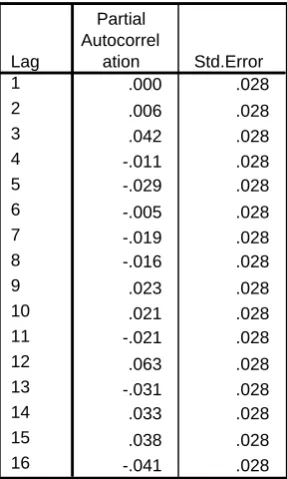
Subsequently, they are shown the total correlograms and partial auto correlations of errors of the variable rain in Caibarién (Table 1 and Table 2), this model was calculated with modeling ARIMA. As it can be appreciated there is a presence of a white noise.

Thus, there is no information in previous steps in the series allowing to predict towards the future, however methodology ROR1is applied to the errors of rain obtaining the following model.

The model explains the 8.7 % of variance; the model has errors of 44.6 mm (Table 3).

Coefficientsa,b

-981.340 308.741 -1.381 -3.179 .003

-795.908 304.288 -1.120 -2.616 .013

7.166 3.007 .374 2.383 .023

.880 .190 .719 4.630 .000

33.632 12.277 1.626 2.739 .010

DI DS NoC Lag3angiostot Lag3XY1 Model 1

B Std. Error

Unstandardized Coefficients

Beta Standardized

Coefficients

t Sig.

Dependent Variable: Angiostotal a.

Linear Regression through the Origin

b. Figure 1 Location of Caibarién station. Villa Clara, Cuba.

Table 1 Correlograms of variable Rain in Caibarién

modeled by ARIMA

In Table 4 it is appreciated that the analysis of

variance is significant with an F of Fisher of 2.5

significant to the 95 %.

In Table 5 it can be appreciated the parameters of

the model. The tendency NoC of errors is to

increase in 0.004 mm, the errors depend on the

errors one month behind (Lag1Error). Although

DI and the tendency NoC are not significant, they

are kept in the model because they provide variance

to the model.

CONCLUSIONS

Through modeling ROR, it can be obtained information for the future projection of data series. This type of modeling opens an important and promising way for the series that behave as a white noise, providing new information for the series and its behavior. The model explains the 8.7 % of variance, with errors of 44.6 mm.

The tendency of errors is to increase around 0.004 mm, although it is not statistically significant, the errors depend on the errors one month behind.

Bibliography

1. Box, G. E. P. and Jenkins, G. M., and Reinsel, G. C., 1994: Time Series Analysis Forecasting and Control, 3rdedition. Prentice–Hall Inc., New Jersey.

2. Centro Meteorológico Provincial Villa Clara

Departamento de Clima

http://meteoweb.vcl.insmet.cu/meteoweb/

3. FIMIA R, OSÉS R, OTERO M, ET AL, (2012). La

malaria. Modelación matemática en el análisis entomoepidemiológico. Evolución de la malaria, modelación matemática y boletines de Vigilancia Epidemiológica en Cuba. Editorial Académica Española, (ISBN 978-3-659-02519-8) for Marca registratada de Academic Publishing GmbH & Co. KGAcademia.

4. FIMIA, R., OSÉS, R., OTERO, M., DIEGUEZ, L.,

CEPERO, O., GONZALEZ, R., SILVEIRA, E., CORONA, E., (2012). El control de mosquitos

(Diptera: Culicidae) utilizando métodos

biomatemáticos en la Provincia de Villa

Clara.REDVET Rev. electrón. vet.

http://www.veterinaria.org/revistas/redvet Volumen

13 Nº 3

-Table 2 Partial self correlograms of the rain in

Caibarién modeled with ARIMA

Table 3 Summary of the model for the series of errors

of rain in Caibarién (xc7) Partial Autocorrelations

Series: Unstandardized Residual

.000 .028

.006 .028

.042 .028

-.011 .028

-.029 .028

-.005 .028

-.019 .028

-.016 .028

.023 .028

.021 .028

-.021 .028

.063 .028

-.031 .028

.033 .028

.038 .028

-.041 .028

Lag 1 2 3 4 5 6 7 8 9 10 11 12 13 14 15 16

Partial Autocorrel

ation Std.Error

Table 4 Analysis of variance of errors modeling

Table 5 Parameters of the model of errors of rain in

http://www.veterinaria.org/revistas/redvet/n03031.h tml.

5. McCracken, D; Dorn, S. (1971). Métodos numéricos

y programación FORTRAN, Edición Revolucionaria. Instituto Cubano del Libro, 1971.

6. OSES R, FIMIA R, SAURA G, PEDRAZA A, RUIZ

N, SOCARRAS J, (2014).Long Term Forecast of

Meteorological Variables in Sancti Spiritus.

CUBA..Applied Ecology and Environmental

Sciences. Volume 2 Number 1 February 2014.ISSN

(Print): 2328-3912, ISSN (Online): 2328-3920. 2014, 2(1), 37-42 DOI: 10.12691/aees-2-1-6.

7. OSES R., FIMIA R,, SILVEIRA, E ,HERNANDEZ

W, SAURA G., PEDRAZA A,GONZALEZ R (2012). Modelación matemática hasta el año 2020 de la densidad larvaria anofelínica de mosquitos (Diptera Culicidae) en Caibarien Provincia de Villa

Clara Cuba .REDVET Rev. electrón. vet.

http://www.veterinaria.org/revistas/redvet Volumen

13 Nº 3

-http://www.veterinaria.org/revistas/redvet/n030312. html.

8. OSES, R. SAURA, G., PEDRAZA, A. a (2012).

Modelación matemática ROR aplicada al

pronóstico de terremotos de gran intensidad en

Cuba,REDVET Rev. electrón. vet.

http://www.veterinaria.org/revistas/redvet.Volumen1

3Nº05B –

http://www.veterinaria.org/revistas/redvet/n050512B .html.

9. OSES, R. SAURA, G., PEDRAZA, A. b (2012).

Modelación de la cantidad de frentes fríos en Cuba, impacto de manchas solares. (2012) REDVET Rev.

electrón. vet. Volumen 13 Nº 05B

-http://www.veterinaria.org/revistas/redvet/n050512 10. OSÉS, R., SAURA, G., OTERO, M.,PEDRAZA, A,

SOCARRAZ, J. RUIZ, N. Cambio climático e impacto en la salud animal en la Provincia de Villa

Clara.CUBA.(2012) Volumen 13 Nº 05B

-http://www.veterinaria.org/revistas/redvet/n050512B. html ,

11. Oses, R.; Grau R. (2011). Modelación regresiva (ROR), versus modelación ARIMA, usando variables dicotómicas en mutaciones del VIH. Universidad Central Marta Abreu de las Villas, 25 de Febrero. Editorial Feijóo. ISBN: 978-959-250-652-7.

12. Oses, R; Fimia, R (2012) Modelos de Pronóstico de Angiostrongilosis y Fasiolósis. Editorial Académica Española,ISBN:978-3-8484-5355-9,.