www.nat-hazards-earth-syst-sci.net/15/1251/2015/ doi:10.5194/nhess-15-1251-2015
© Author(s) 2015. CC Attribution 3.0 License.
Inversion method for initial tsunami waveform reconstruction
V. V. Voronin1, T. A. Voronina2, and V. A. Tcheverda3,4 1Novosibirsk State University, Novosibirsk, Russia
2Institute of Computational Mathematics and Mathematical Geophysics of SB RAS, Novosibirsk, Russia 3A.A.Trofimuk Institute of Petroleum Geology and Geophysics SB RAS, Novosibirsk, Russia
4Kazakh-British Technical University, Almaty, Kazakhstan Correspondence to: T. A. Voronina ([email protected])
Received: 20 November 2014 – Published in Nat. Hazards Earth Syst. Sci. Discuss.: 17 December 2014 Revised: 12 May 2015 – Accepted: 26 May 2015 – Published: 16 June 2015
Abstract. This paper deals with the application of the r -solution method to recover the initial tsunami waveform in a tsunami source area by remote water-level measurements. Wave propagation is considered within the scope of a linear shallow-water theory. An ill-posed inverse problem is reg-ularized by means of least square inversion using a trun-cated SVD (singular value decomposition) approach. The method presented allows one to control instability of the nu-merical solution and to obtain an acceptable result in spite of ill-posedness of the problem. It is shown that the accu-racy of tsunami source reconstruction strongly depends on the signal-to-noise ratio, the azimuthal coverage of recording stations with respect to the source area and bathymetric fea-tures along the wave path. The numerical experiments were carried out with synthetic data and various computational do-mains including a real bathymetry.
1 Introduction
Recently, all of us were witnesses of the terrible tsunami that occurred on 11 March 2011 off the coast of Japan. The tsunami in Japan resembled the disaster in the Indian Ocean in 2004. These mega-events prompted serious efforts to ad-dress the mitigating strategies against the threats posed by tsunamis.
An increasing reliability of tsunami prediction can par-tially be achieved by means of numerical modeling, which makes it possible to estimate the expected propagation, as well as the run up, wave heights and arrival times of a tsunami on the coast that could be subject to risk. An im-portant part of tsunami simulation is to gain some insight
into the tsunami source. The modern tsunami early warn-ing systems conventionally employ seismic methods to de-termine the source parameters. The approaches based on in-version of remote measurements of sea-level data have some advantages because seismic data are not available shortly af-ter an event and are often imprecisely translated to tsunami data. Furthermore, tsunami wave propagation can be simu-lated more precisely than that of seismic waves.
Among the mathematical approaches based on inversion of near-field water-level data are the methods based on Green’s functions technique (GFT) (Satake, 1987, 1989), least square inversion combined with the GFT (Tinti et al., 1996; Piatanesi et al., 2001) and an optimization approach (Pires and Miranda, 2001). A priori information from seis-mic data about a tsunami source played an essential role in the inversion method of Satake. One of the main advantages of the second group of methodologies is that they do not re-quire a priori assumption of a fault plane solution. The first and second approaches are based on the linear shallow wa-ter theory, but the third one allows us to use the nonlinear shallow water equations or other appropriate equation sets. These methods have been widely applied in further studies of tsunami problems with various modifications (Wei et al., 2003).
such combination of unit sub-faults and the real DARTRdata will be as small as possible in a least squares sense.
The developed numerical inversion technique based on least square inversion and truncated SVD (singular value decomposition) approach is here described to reconstruct the initial tsunami waveform (tsunami source) in a tsunami source area based on inversion of remote water-level mea-surements (marigrams). This inversion method was first de-scribed in its fundamentals in the Russian scientific jour-nals (Voronina and Tcheverda, 1998; Voronina, 2004, 2013). Theoretical considerations of such a methodology for a lin-ear long-wave model was discussed by Pires and Miranda (2001).
A direct problem of tsunami wave propagation is consid-ered within the scope of the linear shallow-water theory. Nu-merical simulation is based on a finite difference algorithm on staggered grids. This ill-posed inverse problem of recov-ering initial tsunami waveforms is regularized by means of least square inversion using a truncated SVD approach. As a result of the numerical process an r-solution is obtained (Cheverda and Kostin, 2010). The proposed method allows one to control the numerical instability of the solution and to obtain an acceptable result in spite of the so-called ill-posedness of the problem. The efficiency of the inversion is defined by the relative errors of tsunami source reconstruc-tion. Analysis of the singular spectrum of a matrix obtained allows one to predict the efficiency of inversion by using records produced at a given set of receivers.
One of the substantial advantages of this method is that it is completely independent of any particular source model and its distinguishing feature is the possibility to estimate the capability of a certain observation system to recover the tsunami source.
Based on the properties of the inverse operator studied numerically, we tried to answer the following questions: (1) what minimum number of marigrams should be used to reconstruct a tsunami source well enough; (2) where should the recorders (receivers) of the water-level oscillations be dis-posed relative to potential source area; (3) how accurately can a tsunami source be reconstructed based on recordings with a given monitoring system; (4) is it possible to improve the quality of reconstructing a tsunami source by distinguish-ing the most informative part of the observation system?
In order to answer these questions within the approach proposed, we have carried out a series of numerical exper-iments with synthetic data and different computational do-mains. The results of the numerical simulations have shown a promising outlook of this approach.
2 Models
Mathematically, the problem of recovering the initial tsunami waveform in a source area is formulated as the determina-tion of the spatial distribudetermina-tion of an oscilladetermina-tion source
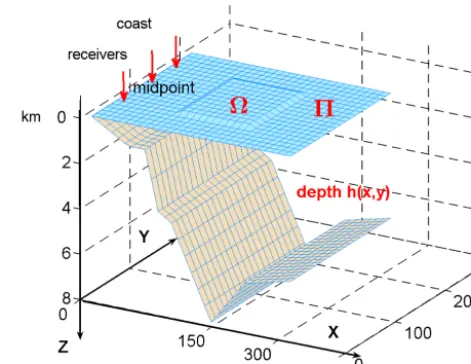
us-Figure 1. The model bottom topography having some basic
mor-phological features typical of the island arc regions.
ing remote measurements on a finite set of points (hereafter called receivers). Let us consider a coordinate systemx y z
and direct the axisz downwards. The plane {z=0} corre-sponds to an undisturbed water surface. The curvature of the Earth is neglected. Let5= {(x;y): 0≤x≤X; 0≤y≤Y}is a rectangular domain on the plane{z=0}. We denote as8
the aquatic part of5with arbitrary solid boundaries0and straight-line sea boundaries.
One of the examples of spatial layout of this statement with straight-line coastal boundaries is represented in Fig. 1 and will be considered in Sect. 5.2. In this case, the domain8
coincides with the domain5. The interaction between the wave and the coast is not considered in this study. Our nu-merical model is based on the shallow water theory. On addi-tion, we look for a solution only in a constrained region. The source area is assumed to be known from seismological data. Let= {(x,y):x1≤x≤xM;y1≤y≤yN}be a tsunami source,⊂8⊆5. Letη(x,y,t )be the function of the wa-ter surface elevation relative to the mean sea level. This func-tion is considered to be a solufunc-tion of the linear shallow water equation:
ηt t =div(gh(x, y)gradη) (1)
with the initial conditions:
η|t=0=ϕ(x, y); ηt|t=0=0 (2)
with the completely reflecting conditions on the continental coasts:
∂η ∂n
0
=0. (3)
the open boundaries. The acceleration of gravity is de-noted as g and the wave phase velocity is defined asc(x,
y)= √
gh(x, y). The tsunami wave is assumed to be trig-gered by a sudden vertical displacement ϕ(x,y) of the sea floor in the target domain. The variableh(x,y) is the wa-ter depth relative to the mean sea level.
The set-up inversion experiments are substantially differ-ent in the functionh(x,y) which varies fromh(x,y)=const to a specialh(x,y)=h(x)modeling the shelf zone and, fi-nally, to the real bathymetry of the Peru subduction zone.
The observational data are water level records which are assumed to be known at a set of points M= {(xi, yi),
i=1, . . . ,P}in the domain8:
η (xi, yi, t )=η0(xi, yi, t ) , (xi, yi)∈M. (4) One can also assume that the set of pointsMbelongs to some lineγwithout self-crossing in the domain8that is necessary only for theoretical purposes.
3 Inversion method
In short, this method is as follows. Let us denote byAthe lin-ear operator of the Cauchy problem presented by Eqs. (1)–(3) and trace its solution on the lineγ (s). Under an appropriate assumption on the functions h(x, y), ϕ(x, y) and the line
γ (s)(this assumption does not necessarily hold in the exper-iments), by means of the standard technique of embedding theorems it was proved (Voronina, 2004, 2012) that the op-eratorA:L2()→L2(γ (s)×(0,T)) is compact and, there-fore, does not possess a bounded inverse. Thus, Eqs. (1)–(3) are now reduced to the following equation:
Aϕ=η0(s, t ), (5)
where
η0(s, t )=η(x(s), y(s), t ), (x(s), y(s))∈γ (s), 0≤t≤T , 0≤s≤L.
As was shown by Kaistrenko (1972), the above inverse prob-lem has a unique solution only if the source function allows factorization in the temporal and spatial variables.
The inverse problem in question can now be formulated as the problem of solving a linear operator equation of the first kind. Its solution will be sought for in a least squares for-mulation. In other words, any attempt to numerically solve Eq. (5) must be followed by a certain regularization pro-cedure. In the present study, regularization is performed by means of truncated SVD that brings about a notion of r -solution (Cheverda and Kostin, 2010).
In brief, the notion ofr-solution can be described as fol-lows: any compact operatorAcan be described in a Hilbert space with a singular system{sj,gj,ej},j=1, . . .∞, where
sj≥0 (s1≥s2≥. . .≥sj≥. . . ) are singular values and{gj},
{ej}are the left and the right singular vectors.A ej=sjgj andsj→0 withj→ ∞. The systems{gj},{ej}are orthog-onal. A very important property of the singular vectors is that they form bases in the data and model spaces, therefore, the solution of Eq. (5) can be given by the expression:
ϕ(x, y)= ∞ X
j=1
η0·gj
sj
ej(x, y). (6)
As one can see from Eq. (6), the ill-posedness of the oper-ator equation of the first kind with compact operoper-ator is due to the fact thatsj→0 withj→ ∞, i.e. one can perturb the right-hand sideη0(s,t )in such a way that its vanishing per-turbation can lead to a large perper-turbation of the solution.
The regularization procedure based on truncated SVD leads to a notion ofr-solution given by the formula
ϕ[r](x, y)=
r X
j=1
η0·gj
sj
ej(x, y). (7)
Anr-solution is the projection of the exact solution of Eq. (6) onto a linear span ofrright singular vectors corresponding to the top singular values of the compact operatorA. This trun-cated series is stable for any fixed parameterr with respect to perturbations of the right-hand side and the operator as it is (Cheverda and Kostin, 2010). The value ofris determined by the formula
r=max{k:sk/s1≥1/cond}, (8)
where cond=cond(A) is set by the user restriction on the conditioning number of the matrix A. It is clear that the value ofrdepends on the rate of decreasing of singular spectrum of the matrix A, which is tightly bounded with the parameters of the observation system and noisiness of data. Indeed, let us assume the perturbation in the right-hand sideη0(s,t) is known and can be written in the form
ε(t )=
L X
j=1
εj(t )gj,
then the perturbed solution will be represented as
ϕ[r](x, y)=
r X
j=1
(η0+ε)·gj
sj
ej(x, y). (9)
One should limit the upper index in the last sum from the time whensj is far lessεj(t )to avoid the numerical insta-bility. It is reasonable that the larger theris, the more infor-mative the solution will be. Note that the fitted value ofris much less than a minimum of the matrix dimensions.
4 Finite dimensional approximation andr-solution In a real situation, one can numerically resolve only a finite dimensional subsystem of Eq. (5) with (K×L) submatrix. Convergence of ther-solution of a finite-dimensional system of linear algebraic equations to ther-solution of an operator equation was carefully investigated by Cheverda and Kostin (2010).
To solve numerically Eqs. (1)-(3) we applied a finite dif-ference approach for its equivalent first order linear system in terms of the unknown water elevationη(x, y, t )and velocity vectorV:
ηt+g∇ ·(hV)=0
Vt+g∇η=0 (10)
completed by the following initial conditions:
η|t=0=ϕ(x, y),V|t=0=0; (11)
and the boundary condition on the solid boundary:
V·n=0 (12)
and absorbing conditions on the open boundaries. This prob-lem was approximated by an explicit–implicit four-point fi-nite difference scheme on a uniform rectangular grid which is based on the staggered grid stencil using the central-difference approximation of spatial derivatives. As it was mentioned above, the wave run up is not considered in this study, hence we infer the coast line when the depth h(x,
y)=50 m.
In order to obtain a system of linear algebraic equations by means of the projective method, a trigonometric basis was chosen in the model space, i.e. the unknown function of wa-ter surface elevation ϕ(x, y) is approximated in the target domain(Sect. 2) by a sum of spatial harmonics{ϕmn(x,
y)=sinmπl
1 (x−x1)·sin nπ
l2 (y−y1)} with unknown coeffi-cientsc= {cmn}:
ϕ(x, y)=
M X
m=1 N X
n=1
cmnϕmn(x, y), (13)
the center of the tsunami source was believed to be at a point (xc,yc) being the central point of the domainand
l1=(xM−x1);l2=(yN−y1). We assumed the water level oscillations η0(x, y, t) are known at a set of points {(xp,
yp)},p=1, . . . ,P for a finite number of time samples{tj},
j=1, . . . ,Nt, i.e.
η0= η11, η12, . . ., η1Nt, η21, . . ., η2Nt, ηP1, . . ., ηP Nt T
,
ηpj =η0 xp, yp, tj
.
The unknown functionϕ(x,y) was sought for according to Eq. (13).
Now, we assume that the dimensions of the solution and the data space are equal to:
dim(sol)=K=M×N; dim(data)=L=P×Nt. In the end, a linear algebraic system for the unknown vectorc
of coefficients{cmn}(ordered in any one-dimensional way) from Eq. (13) was obtained:
η0=Ac, (14)
where A is a matrix whose columns consist of computed waveforms in every receiver for each spatial harmonic used as the source,η0is a vector containing the observed tsunami waveforms. Now, the matrix A is ofKbyLmatrix. After the SVD procedure one could obtain the singular values of the matrix A, its left and right singular vectors{gi,i=1, . . . ,L},
{ek,k=1, . . . ,K}. The valuercould be fitted by analyzing the singular spectrum of the matrix A.
Then ther-solution of Eq. (14) is represented by the sum
c[r]=
r X
j=1
αjej, (15)
where{αj= (η0,gj)
sj }and{gj},{ej}are the left and the right singular vectors of the matrix A,{sj}are its singular values.
Finally, the numerical simulation includes the following steps:
1. First, we obtain synthetic marigrams in all receivers by solving the forward problem with a certain function
ϕ(x,y) as a source to be reconstructed. Thus, the vector
η0in Eq. (14) is obtained.
2. The computed marigrams are perturbed by a back-ground noise, i.e. a high-frequency disturbance and ap-propriate filtering is applied.
3. Next, the matrix A is numerically computed by solving the forward problem with every spatial harmonic{ϕmn},
m=1, . . . ,M;n=1, . . . ,Nas a source.
4. Further, the standard SVD procedure is applied. The analysis of singular spectrum of the matrix A allows one to choose the numberr varying the conditioning number of the matrix A, as was explained above, and to compute the coefficients{cmn}by solving Eq. (14). 5. After this, the functionϕ(x,y) can be computed
accord-ing to Eq. (13).
6. To estimate the efficiency of the inversion experiment we use a misfit parameter which is defined as a relative
L2-error by the formula: err%=|ϕ− ˆϕ|L2()
|ϕ|L2() ×100 %.
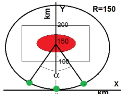
Figure 2. A layout scheme of the source-receivers arrangement in
Model 5.1.
5 Numerical experiments: description and discussion A series of calculations has been carried out by the method proposed to clarify the dependence of the efficiency of the inversion on certain characteristics of the observation system such as the number of receivers and their location, frequency or temporal range of data and the signal-to-noise ratio. We postulate that source area is given, as it is in real cases. Synthetic data for the numerical inversion experiments pre-sented below were computed as a solution of Eqs. (10)–(12) with respective open boundary conditions. In addition, the functionϕ(x,y) was explained by the relation:
ϕ(x, y)=β(x, y)·α(x), (16)
where functionβ(x,y) makes a semi-ellipsoid with the cen-ter at the point (x0, y0) and the radii Rx and Ry on the planez=0. The parameterα(x)is perturbation of this semi-ellipsoid. Whenα(x)=1 the initial tsunami waveform was assumed to be a semi-ellipsoid or a semi-sphere.
5.1 Case studyh(x,y)=const
Firstly, to avoid the influence of such factors as bathymetry and data noise, we consider a formal calculation domain with open boundaries, with the depthh(x,y)=h0, the wave phase velocity c(x,y)=√g h0=c0 andα(x)=1. The setting of the problem allows us to consider our problem in the spectral domain and to use ther-solution method for analytical solu-tion (Voronina and Tcheverda, 1998; Voronina et al., 2014). The basic properties of the inverse operator were numerically studied.
In short, we have shown that the inversion results are bet-ter when the aperture length is rising, increasing the upper limit of the frequency band makes the obligatory effect for the inversion quality and leads to decreasing the smearing of the recovered function and, hence, to increasing extreme val-ues in the center of the source. The results of the inversion
by a wide angle aperture coincide with the experiments on a wide linear aperture. It was shown, if receivers were uni-formly distributed along the linear aperture, the efficiency of the inversion was improving when the number of receivers increases up to 15 but further increasing the receivers number was useless. The receivers-to-source distance has no effect on the inversion result in the case studied. If the number of receivers is fixed the efficiency of the inversion rises with the azimuthal coverage. We have shown that a more precise def-inition of the target domain relative to the size of a tsunami source leads to a decrease in the number of necessary re-ceivers, perhaps as little as 5–7. In addition, the released en-ergy as well as the maximum value of the recovered function increases. However, the total volume of water displaced due to the source in the domainis not varied.
The results obtained allowed us to outline the main details of the methodology proposed. The basic point is that analyz-ing a sanalyz-ingular spectrum of the obtained matrix A enables us to make an assumption about the forthcoming efficiency of the inversion.
Let us see how that works in the context of the dependence of the efficiency of the inversion on the number of receivers and their azimuthal coverage. Our numerical experiments were conducted with the fol-lowing parameters (in spectral domain): = {(x, y):
−100 km≤x≤100 km; 100 km≤y≤200 km}, frequency
w∈[0.001, 0.01] Hz; α(x)=1 in Eq. (16), i.e. the type of the source is a semi-ellipsoid withRx=50 km;Ry=25 km and the center was assumed at the point (x0,y0)=(0.150) ac-cording to Fig. 2. The conditioning number of the matrix A was 108in all calculations that is possible due noise-free syn-thetic data. Let us define an above assembly of the fault pa-rameters as Model 5.1. Our purpose was to obtain accept-able results of the inversion using a minimum of marigrams, so, we made a computer simulation when the number of re-ceivers ranged from one to five when they were placed on the circle aperture with the different aperture angle. Figure 2 shows a layout scheme of the source-receivers arrangement in Model 5.1.
We will use the following notations: (1) the conditioning number of the matrix A is designated as cond. (A); (2) the value 100×max (ϕ(x,y)), while (x,y)∈is denoted by the symbol{100max}; (3) the misfit parameter is denoted by err %.
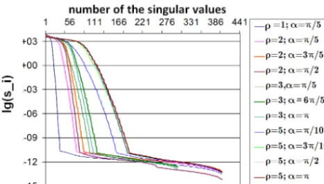
The common logarithms of singular values for these nu-merical experiments are plotted in Fig. 3. A sharp decrease in the singular values, when their number increases, is typ-ical for all calculations in all cases of the study, due to the ill-posedness of the problem.
Figure 3. The dependence of singular values of the matrix A ( in
logarithmic scale) on their numbers;ρ denotes the number of re-ceivers used in the inversion and arranged on the aperture with angle equal toα.
As will be clear below, increasing the number of records alone does not lead to a good inversion if there is insufficient azimuthal coverage with respect to the source and, on the contrary, in real cases it turns out that the noisiness of data is raised resulting in lower efficiency of inversion.
Indeed, in Fig. 4 one can see how the numberr (the blue line) and a maximum value of the recovered function (the red line) varied on the number of receivers used (down horizon-tal axis) and on the aperture angle (upper horizonhorizon-tal axis). One can see from these graphs that increasing the number of receivers, in total, leads to a better inversion: misfit pa-rameter (the green line) decreases by increasing the number of receivers used, as well as maximum value of the recov-ered function tends to a maximum value of the theoretical function. If the number of receivers is fixed, the efficiency of inversion rises with the azimuthal coverage that has a good matching with our previous assumption based on analyzing singular spectra. We have also shown that if the aperture angle is sufficiently wide, the influence of the conditioning number is not significant, but the inversion parameters are worse for a smaller conditioning number of the matrix A. The recovered functions for the cases discussed above are presented in Figs. 5–6.
5.2 Case studyh(x,y)=h(x)
How does a bottom relief and a more realistic type of the source influence the inversion result? To answer this question we have carried out numerical experiments for the model bot-tom topography having some basic morphological features typical of the island arc regions (see Fig. 1).
As the initial sea surface displacement, a sea floor de-formation of typical tsunamigenic earthquakes with reverse dip-slip or low-angle trust mechanisms was used. Its dipolar shape was simulated according to Eq. (16) with the param-eterα(x)=(x−x0+3·R1)·(x−x0+R1/6); andR1=25;
R2=50 (see Fig. 14, left panels). The target domainwas
Figure 4. The parameters of the inversion using 1, 2, 3, 5 receivers:
100 max symbolizes maximum value of the recovered function mul-tiplied by 100 (the red line), the values of numberr(the blue line) and the misfit parameter err % (the green line).
a rectangle{(x,y): ∈[100; 200]×[50; 150]}, the calcula-tion domain was a rectangle5= {(x, y): ∈[0; 300]×[0; 200]}, the center point of the tsunami source was placed at (x0;y0)=(150; 100) (see Fig. 1).
Synthetic data for the numerical inversion experiments presented below were computed as a solution of Eqs. (10)– (11). The full reflection boundary condition described in Eq. (12) is fulfilled on the coast linex=0 and the absorbing boundary conditions are imposed on the open free bound-aries:
cηyt+ηt t+
c2
2ηxx=0, (x, y)∈y=0;
−cηyt+ηt t+
c2
2ηxx=0, (x, y)∈y=200;
−cηxt+ηt t+
c2
2ηyy=0, (x, y)∈x=300.
The functionϕ(x,y) was sought for according to Eq. (13) withM=25,N=11. Synthetic marigrams were calculated forNt=1990 time instants. Receivers were disposed on the segment [10; 190] of the linex=0, i.e. a maximum of the aperture length was 180.
As in the previous case with a constant depth of the calcu-lated basin we tried to use a minimum number of marigrams in the inversion process. For this reason, the parameterP was equal to 1, 2, 3, 5. Some aspects of this study were presented in Voronina (2004). We now turn to these models to make a generalization. The point in question is the location of re-ceivers with respect to the dipolar source.
seg-Figure 5. The recovered functions using 2 (left panels), 3 (middle panels), 5 (right panels) receivers located on the circle aperture with
aperture angle equal toα=π/5 (left panels, middle panels) and toα=π/10 (right panels), respectively.
Figure 6. The recovered functions using 2 (left panels), 3 (middle panels), 5 (right panels) receivers located respectively on the circle aperture
with aperture angle equal toα=π.
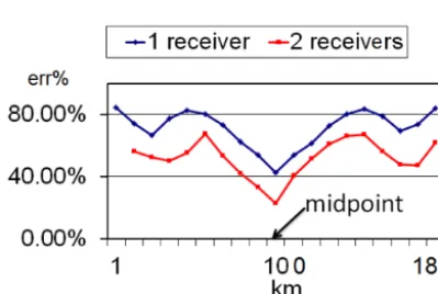
Figure 7. The misfit parameter err % in terms of the position f
re-ceivers on the aperture: with one receiver used (the blue line); with two receivers (the red line).
ment stopping every 10 km along the linex=0 with coordi-nates (0, 10n) according to the coordinate system of Fig. 1. Hence, the length of aperture in every position is equal to 10n,n=1, . . . , 19.
The most important information that should be drawn from these graphs points to the presence of an obvious minimum of the functions presented. One can see points of a minimum in these graphs corresponding to the experiments with the re-ceiver disposed at midpoint. In other words, availability of waveform from this observation point significantly improves the inversion result. The following numerical experiments confirm this inference.
A substantial decrease of the misfit parameter when re-ceivers are placed at the midpoint can be explained by the dipolar shape of the source and, hence, the signal in this di-rection is mostly informative.
For this reason, in the following experiments with three and five receivers, one of receivers is always fixed at the mid-point. The conditioning number of the matrix A was equal to 100 in the experiments below.
Now, synthetic waveforms were simulated as a result of the solution to the direct problem described in Eqs. (10)– (11) perturbed by the background noise, consisting in a high-frequency disturbance about 5 % rate of a maximum signal amplitude over all the receivers. Admittedly, we did not ob-tain any appropriate result with perturbed synthetic data due the ill-posedness of the problem. However, since a tsunami wave is more lower frequency compared to the background noise, it is reasonable to apply the frequency filtration of an observation signal. In this paper, filtration is done by a method of grid function smoothing proposed by V. A. Tset-sokho and A. S. Belonosov in 1976. The description of this method can be found in Yurchenko et al. (2013).
Figure 8. The inversion parameters for the Case1 (three receivers)
and Case2.2 (five receivers). Aperture located symmetrically with respect to midpoint. The yellow color of columns denote that the aperture is placed inside the segment of the coast line corresponding to the projection of the source on the coast.
We have considered the following versions of the receivers disposition:
– Case1: an observation system of three receivers. One receiver is always placed at the midpoint but two other receivers are symmetrically placed with respect to the midpoint with distances 10n,n=1, . . . , 9 every step. – Case2: an observation system of five receivers. Again,
one receiver is always placed at the midpoint, two pairs of receivers moved symmetrically from the cen-ter to the endpoints of the aperture, while a distance between every nearest-neighbor receivers in every pair was fixed as 40 km (the case named C2.1), 20 km (the case named C2.2) and 10 km (C2.3).
There is an aperture length on the horizontal axis in Fig. 8. The parameters of the inversion for Case 1 as functions of the aperture length are presented in Fig. 8. The misfit parameter err % (the blue line) is decreasing but maximum and mini-mum values of the recovered function (the orange and the brown lines, respectively) converge to the corresponding val-ues of the initial function (the red lines) at the moment when the aperture length approaches the projection of a source on the aperture line that corresponds to the yellow columns in Fig. 8.
These regularities remain valid for the inversion with five waveforms. Indeed, the behavior of the 100max (the magenta line) and err % (the dark magenta line) for case C2.2 is sim-ilar to the ones of case C1 and bears witness to better results of the inversion.
Case C2.2 differs from case C2.3 by a more uniform dis-tribution of the same number of receivers within the acting aperture segment being the projection of the source on the aperture line that leads to improving the inversion parame-ters. By comparing the values of parameters in the yellow and light-blue columns in Fig. 8 one can conclude that a fur-ther increase in the aperture length leads to worse results.
The importance of the receiver location at the midpoint was confirmed in these series of numerical experiments, too. As was shown, replacing the central point of a set of receivers from the midpoint results in increasing the misfit parameter and, at the same time, in decreasing the maximum value of the recovered function. In other words, we lose the most in-formative waveform.
As an example, the recovered functions corresponding to the inversion for Case 1 and Case 2.2 are presented in Fig. 9 (middle-right and right panels). From the graphs of singular spectra of the inversions with three and five waveforms plot-ted in Fig. 9 (left panel) one can expect that the inversion in the latter case will be more successful. Indeed, results of numerical experiments presented in Fig. 9 (middle, right pan-els) substantiate our assumption based on analyzing singular spectra.
It is now clear that the quality of inversion strongly de-pends on the disposition, the number of receivers and noisy data. The robust result could be obtained when, at least, one of the receivers involved is placed at the midpoint which is a projection of the major variability direction of the source. 5.3 Case study: real bathymetry of the Peru
subduction zone
Finally, to illustrate some of the ideas let us consider the re-sults obtained for the case study with the real bathymetry of the Peru subduction zone. We are interested in how distinc-tive features of a real bathymetry affect the inversion pro-cess. The simulation area is located from 85 to 71◦W and from 5 to 15◦S. We set up the following parameters for our calculations: the domain8 was the aquatic part of a rect-angle5= {0≤x≤600; 0≤y≤400}with piecewise-linear boundaries of the dry land, the domain{= {400≤x≤500; 200≤y≤300}(see Fig. 10). As mentioned above, the wave run up was not considered. The observed data were simulated as a solution of Eqs. (10)–(12) and completed with the full absorbing boundary conditions of second order of accuracy being fulfilled on the open boundaries.
Again, as an initial sea surface elevation, the sea floor de-formation of typical tsunamigenic earthquakes with reverse dip-slip or low-angle thrust mechanisms was used and it is plotted in Fig. 14 (left panel) with the following parame-ters: the center point (x0; y0)=(450; 250), maximum and minimum values of initial displacement in source areaϕ(x,
y) ϕmax=1.959 m;ϕmin= −0.67 m. As before, we tried to obtain acceptable results of the inversion using a minimum number of records. In our calculations, the functionϕ(x,y) was sought for according to Eq. (13) withM=25,N=11. These values are defined by the shape of theoretical function
Figure 9. The dependence of singular values of the matrix A (in logarithmic scale) on their numbers when three (the blue line) and five
(the red line) receivers are used in the inversion (left panel). The recovered function with (25×11) exact coefficients according to Eq. (13) withϕmax=0.73 m,ϕmin=0.34 m in target domain (middle left panel).The recovered function when three waveforms were used in the inversion: err %=37.1 %;ϕˆmax=0.63 m;ϕˆmin= −0.282 m; length of aperture.=80 km; (middle right panel). The recovered function when five waveforms were used: err %=20.4 %;ϕˆmax=0.71 m;ϕˆmin= −0.289 m; length of aperture.=140 km (right panel).
Figure 10. Isolines of the Peru subduction zone with depth values
(in km), the target domain and 14 receivers marked by the green color symbols (◦).
reach all receivers, specifically, the number of time steps was
Nt=1684 in the case presented.
After specifying all the parameters we carried out the steps of the numerical simulation mentioned in Sect. 4. Synthetic marigrams were perturbed by the background noise with the disturbance rate about 3 % of a signal maximum amplitude over all the receivers. It is imperative that the filtration pro-cedure was made after the noise pollution. Next, the standard SVD-procedure was performed and the singular spectrum of the matrix A was obtained.
As before, first of all we analyzed the singular spectrum of the matrix A. For example, the graphs of the common loga-rithm of the singular values of the matrix A corresponding to their numbers are presented in Fig. 11. for the inversion with three (the red line), four (the blue line), nine (the magenta line) and ten (the green line) waveforms used in the calcu-lations. Comparing singular spectra for the inversion with some sets of three and four marigrams in Fig. 11, one can assume that such an increase in the number of receivers will lead to the deterioration of the solution. Inversion parameters
Figure 11. Typical graphs (upper parts) of singular values in the
common logarithm scale of the matrix A with respect to their num-bers when the number of waveforms used in the inversion is equal to three (the red line), four (the blue line), nine (the magenta line) and ten (the green line).
corresponding to these cases are presented in Table 1 (the first and the fifth rows).
We have seen, until now, that adding new receivers always led to better solutions when a depth of the calculation basin was a synthetic function. However, this prediction is not uni-versally true for the case with a real bathymetry. Only in-creasing the number of receivers without considering their azimuthal coverage could result in a worse inversion due to rising a general level of noise pollution of data.
Obviously, the parameterrshould be taken only from the first interval, where the common logarithms of singular val-ues are slightly sloping because further increases in numberr
leads to the solution instability. On the other hand,rshould be large enough to provide a suitable spatial approximation ofϕ(x,y). From the numerical experiments it is clear that a satisfactory parameter value hasr≥70 (Voronina, 2012).
Table 1. The inversion parameters with sets of used receivers.
P Cond r Err % ϕmax ϕmin Receivers
3 100 41 71.7 1.213 −0.78 3, 10, 12
3 1000 42 74.8 1.577 −1.55 3, 10, 12
4 100 15 74.22 0.892 −0.655 3, 4, 12, 13 4 1000 16 75.22 0.905 −0.647 3, 4, 12, 13
4 100 34 99.1 0.128 −0.107 3, 4, 5, 7
4 100 34 65.86 0.419 −0.156 2, 6, 10, 14
5 100 45 62.3 1.185 −0.67 3, 4, 6, 7, 11
5 1000 57 40.9 1.699 −0.75 3, 4, 6, 7, 11
5 1000 16 74 0.845 −0.69 3, 4, 6, 7, 9
9 100 73 37.7 1.539 −0.72 3, 4, 5, 6, 7, 8, 9, 10, 11 9 1000 104 63.3 2.396 −1.29 3, 4, 5, 6, 7, 8, 9, 10, 11 9 1000 104 59.9 2.25 −1.04 3, 4, 5, 9, 10, 11, 12, 13, 14
10 100 72 37.24 1.545 −0.645 3, 4, 5, 6, 7, 8, 9, 10, 11, 12 10 1000 99 86.75 2.632 −1.909 3, 4, 5, 6, 7, 8, 9, 10, 11, 12 10 1000 15 62.9 1.099 −0.74 1, 2, 3, 5, 6, 7, 9, 12, 13, 14
The number of receivers used in the inversion process is denoted byP. Maximum and minimum values
of the recovered function are symbolized byϕˆmaxandϕˆminrespectively (scaled in meters) The
dimension of the subspace where the exact solution was projected is symbolized byr. The conditioning number of the matrix A is denoted by cond and the misfit parameter is denoted by err %.
Figure 12. Singular spectra in the common logarithm scale for the
models: V1.1 and V1.2 (the brown line), V2.1 and V2.2 (the red line); V3.1 and V3.2 (the blue line), V4 (the green line) (see Ta-ble 2).
played by locating the monitoring system relative to the to-pography and source area.
Indeed, adding to the observation system the receivers with numbers {12, 13, 14}(see the 12th and the 15th row in Table 1) which were not affected by disturbance due to the reflection from the underwater vertical ledge, did not im-prove the solution, according to the expectations. The same is true for a set of receivers {1, 2, 3, 4}which, on the con-trary, were placed in the direction where the distortion of the signal is more possible due to the features of the relief. Us-ing receivers with numbers {5, 6, 7, 8, 9, 10, 11}one can obtain a strong improvement of the inversion. The replace-ment of even one or two of them leads to a solution
deteri-oration (see the eighth and the ninth rows in Table 1). What are the odds? It seems reasonable to say that the matter is in the dipole shape of our source and in the existence of a cer-tain angle between its axis and the line of the reflection (the coast line and the underwater ledge). The axis of the source in our case is directed along the axisx and is not perpendic-ular to the coast line like in the previous model. The latter set of receivers is distributed along the reflection ray corre-sponding to the direction of the strongest variability of the source. It should be remarked that the use of all the receivers does not improve the inversion because this set of marigrams involves many fewer informative waveforms that only leads to increasing the noisy pollution of the data.
The last series of the numerical experiments was aimed at finding out the most informative direction of the receivers location in terms of improving the inversion. We have chosen several sets each consisting of seven receivers differing in their location.
The upper parts of singular spectra for these numerical ex-periments are plotted in common logarithm scale in Fig. 12. It is also shown in Fig. 12, how one could define the numberr
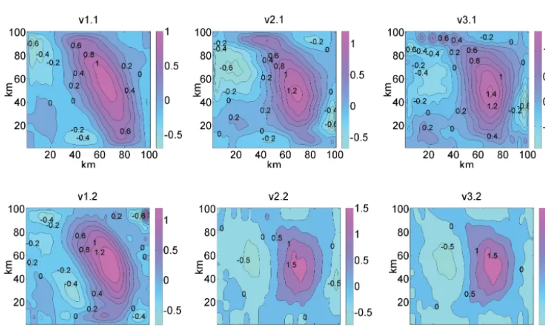
for every settled conditioning number of the matrix A. In Table 2 one can see the major parameters of the inver-sion with seven marigrams by Models V1–V4 which differ in the receivers location and the conditioning number of the matrix A.
Table 2. The inversion parameters for different sets with seven receivers.
Model Cond r Err % ϕmax ϕmin Receivers
V1.1 100 23 62.8 1.106 −0.696 3, 4, 5, 6, 7, 8, 9 V1.2 10 000 32 51.9 1.392 −0.49 3, 4, 5, 6, 7, 8, 9
V2.1 100 73 37.7 1.559 −0.717 3, 4, 5, 6, 9, 10, 11 V2.2 10 000 92 32.7 1.686 −0.735 3, 4, 5, 6, 9, 10, 11
V3.1 100 65 45.9 1.449 −0.923 5, 6, 7, 8, 9, 10, 11 V3.2 10 000 104 26.7 1.816 −0.703 5, 6, 7, 8, 9, 10, 11
V4 10 000 59 31.73 1.706 −0.737 1, 3, 5, 7, 9, 11, 13
Maximum and minimum values of the recovered function are denoted byϕˆmaxandϕˆmin
respectively (scaled in meters). The dimension of the subspace where the exact solution was projected is symbolized byr. The conditioning number of the matrix A is denoted by cond and the misfit parameter is denoted by err %.
Figure 13. The recovered functions: cond(A)=100 (top panels) by models V1.1 (left panel), V2.1 (middle panel) and V3.1 (right panel); cond(A)=10000 (bottom panels) by models V1.2 (left panel), V2.2 (middle panel) and V3.2 (right panel).
a lesser smearing effect in the shape of the recovered func-tion.
It should be noted that the misfit parameter gives only a global estimation of the efficiency of the inversion. Based on our experiments with perturbed data and a real bathymetry we can conclude that the value of the misfit parameter err %≈20–26 % allows us to obtain a robust shape of the recovered source. In Fig. 14 the theoretical functionϕ(x,y) and the one recovered by model V3.2 are presented. The ex-treme values of the recovered function have changed due to smoothing.
After the inversion by model V3.2 was completed, we again solved the direct problem with the recovered and smoothed functionϕ(xˆ ,y) and calculated marigrams at the
Figure 14. Theoretical source model: ϕmax=1.959 m; ϕmin= −0.67 m (left panel). Model V3.2ϕˆmax=1.816 (1.514) m;
ˆ
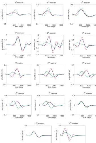
Figure 15. Comparison between theoretical (the red line) and calculated waveforms in all receivers: the green line indicates the waveform
computed using the source reconstructed with 5 receivers{3, 4, 6, 7, 10}; the blue line indicates the waveform computed using the source reconstructed with 7 receivers{5, 6, 7, 8, 9, 10, 11}; the time increment equals 3 s.
same 14 points. Marigrams computed with the recovered tsunami source have a good matching with the initial syn-thetic ones not only in seven receivers used in the inversion process but also in all 14 receivers as well (see Fig. 15).
This fact can be treated as a verification of the inversion algorithm. In addition, the coincidence of marigrams has a
6 Conclusions
We have applied an approach based on SVD andr-solution methods to recovering the initial tsunami waveform in a tsunami source area.
Searching for the initial water surface displacement as a series of spatial harmonics is a common practice; however, the method proposed allows one to control the numerical in-stability by tools of the r-solution method. The value r is essentially determined by a real bathymetry, spatial location of the observation system, the data noisiness and still it is significantly less than the dimension of the matrix obtained in the calculations. By analyzing the singular spectrum of the matrix it is possible to make a preliminary prediction of the efficiency of the inversion with a given set of the recording stations. Hence, we could make a well-aimed precomputa-tion with varying locaprecomputa-tions of candidate receivers to obtain the best inversion possibly in a real process. This potential of the method should be kept in mind when designing a moni-toring system for tsunamis.
By the numerical simulations we have shown that in order to obtain a reasonable quality of the source restoration we need at least five to seven receivers in the simulation with a real bathymetry. Reconstructing the shape of a source is im-proved when not only the number of receivers increases but their azimuthal coverage with respect to a source area im-proves as well. The receivers-to-source distance does not es-sentially influence the inversion result. One of the advantages of the method proposed is that it is completely independent of any particular shape of a source, however, a limitation of this method is that it is suitable only for the linear theory.
The location of receivers on direct and reflected rays cor-responding to the direction of the strongest variability of the dipole source have the greatest effect for the inversion result. As is shown in the numerical experiments, it is this set of re-ceivers that provides the best results of the inversion process.
Acknowledgements. Vladimir Tcheverda was partially supported by the Ministry of Education and Science of the Republic of Kazakhstan grants 0981/GS4 and 1771/GS4.
Edited by: A. Armigliato
Reviewed by: three anonymous referees
References
Cheverda, V. A. and Kostin, V. I.: r-pseudoinverse for compact op-erator, Siber. Elect. Math. Rep., 7, 258–282, 2010.
Enquist, B. and Majda, A.: Absorbing boundary conditions for the numerical simulation of waves, Math. Comp., 139, 629–654, 1977.
Kaistrenko, V. M.: Inverse problem for reconstruction of tsunami source, Tsunami Waves, Proc. Sakhalin Compl. Inst., 29, 82–92, 1972.
Lavrentiev, M. M. and Romanenko, A. A.: Tsunami Wave Parame-ters Calculation before the Wave Approaches Coastal Line Pro-ceedings of the Twenty-fourth (2014) International Ocean and Polar Engineering Conference, 15–20 June 2014, Busan, Korea, 96–102, 2014.
Percival, D. B., Denbo, D. W., Eble, M. C., Gica, E., Mofjeld, H. O., Spillane, M. C., Tang, L., and Titov, V. V.: Extraction of tsunami source coefficients via inversion of DARTr buoy data, Nat. Haz-ards, 58, 567–590, 2011.
Piatanesi, A., Tinti, S., and Pagnoni, G.: Tsunami waveform in-version by numerical finite-elements Green’s functions, Nat. Hazards Earth Syst. Sci., 1, 187–194, doi:10.5194/nhess-1-187-2001, 2001.
Pires, C. and Miranda, P. M. A.: Tsunami waveform inversion by adjont methods, J. Geophys. Res., 106, 19773–19796, 2001. Satake. K.: Inversion of tsunami waveforms for the estimation of a
fault heterogeneity: method and numerical experiments, J. Phys. Earth, 35, 241–254, 1987.
Satake, K.: Inversion of tsunami waveforms for the estimation of heterogeneous fault motion of large submarine earthquakes: the 1968 Tokachi-oki and the 1983 Japan sea earthquake, J. Geo-phys. Res., 94, 5627–5636, 1989.
Tinti, S., Piatanesi, A., and Bortolucci, E.: The finite-element wave-propagator approach and the tsunami inversion problem, J. Phys. Chem. Earth, 12, 27–32, 1996.
Voronina, T. A.: Determination of spatial distribution of oscillation sources by remote measurements on a finite set of points, Sib. J. Calc. Math., 3, 203–211, 2004.
Voronina, T. A.: Reconstruction of Initial Tsunami Waveforms by a Trancated SVD Method, J. Inverse and Ill-posed Problems, 19, 615-629, 2012.
Voronina, T. A.: Application of r-solutions to reconstructing an ini-tial tsunami waveform, Numerical methods and Programming, Scient. On-line Open Access J., 14, 165–174, 2013.
Voronina, T. A. and Tcheverda, V. A.: Reconstruction of tsunami initial form via level oscillation, Bull. Nov. Comp. Center, Math. Model. Geoph., 4, 127–136, 1998.
Voronina, T. A., Tcheverda, V. A., and Voronin, V. V.: Some prop-erties of the inverse operator for a tsunami source recovery, Siberian Electronic Mathematical Reports, http://semr.math.nsc. ru (last access: 10 June 2015), 2014.
Wei, Y., Cheung, K. F., Curitis, G. D., and McCreery, C. S.: Inver-sion algorithm for tsunami forecast, J. Waterw. Port Coast. Ocean Eng., 129, 60–69, 2003.