Nat. Hazards Earth Syst. Sci., 10, 1689–1695, 2010 www.nat-hazards-earth-syst-sci.net/10/1689/2010/ doi:10.5194/nhess-10-1689-2010
© Author(s) 2010. CC Attribution 3.0 License.
Natural Hazards
and Earth
System Sciences
On the application of kinematic models to simulate the diffusive
processes of debris flows
M. Arattano1and L. Franzi2
1Research National Council, Torino, Italy
2Public works, soil defence department, Regione Piemonte, Torino, Italy
Received: 19 November 2009 – Revised: 26 April 2010 – Accepted: 12 May 2010 – Published: 18 August 2010
Abstract. Debris flows generally propagate along steep mountain torrents with dynamics primarily governed by gravitational and frictional forces. Thus, debris flows mod-elling can be successfully performed through the application of kinematic models, which consider only the effects of slope and friction and neglect the remaining terms of the momen-tum equation. However, the diffusion processes that can be observed in the field, such as the spreading of the debris flow wave as it flows downstream, can not be theoretically pre-dicted by kinematic models, since diffusion is a second-order process neglected in the kinematic approximation. In this paper, this issue is discussed and an application for both a generalized diffusion wave model and a kinematic model is proposed of a debris flow which occurred in an Italian in-strumented torrent to identify, in a real case scenario, the effective value of the neglected terms in the kinematic ap-proximation.
1 Introduction
Debris flows usually occur in mountain torrents characterised by steep channel slopes. Debris flows may significantly dif-fer as far as the number of surges following the main wave (or superimposed to it), maximum discharge, front height and magnitude are concerned. These general characteristics may vary from case to case, depending on triggering con-ditions, channel geometry and the rheology of the mixture (Takahashi, 1991). Nevertheless, debris flows share some similarities. In particular, debris flows show two diffusive characteristics as they travel downstream:
1. spreading of the hydrograph;
Correspondence to: M. Arattano
2. decay of front height (Pierson, 1986; Johnson, 1970; Genevois et al., 2000; Arattano and Marchi, 2008; Iver-son, 1997; H¨urlimann et a., 2003).
Similar characteristics can also be observed in flume ex-periments performed to simulate debris flow mechanics (Pu-dasaini et al., 2005; Lanzoni and Tubino, 1993). The reduc-tion of the front height and the spreading of the debris flow hydrograph may also be observed for lahars (Pierson et al., 1990).
Mathematical models are commonly employed to simu-late the propagation of debris flows along the torrent and predict the front height evolution, the hydrograph deforma-tion and then the deposideforma-tion on the fan. The simuladeforma-tion of the propagation phase of the flow within the channel bound-aries is normally performed through 1-D models, using the so called Saint-Venant equations, while the deposition is simu-lated through 2-D models.
the process, but they cannot dissipate their discharge or flow stage. Therefore, the effective capability of kinematic mod-els to simulate real debris flows and their observable diffu-sive characteristics as they travel downstream, as in the case of the Arattano and Savage (1994) model, should be better understood and explained. Moreover, the effect of the dif-fusive terms should be quantified to verify its amount and a discussion is needed about the possibility to adequately sim-ulate debris-flow processes through kinematic models.
2 The kinematic model
Modelling a water-sediment flow on a steep slope is gener-ally made using the Saint-Venant equations, which are ob-tained by assuming a hydrostatic pressure distribution over the flow depth, no erosions and depositions and slowly vary-ing cross-sections. The Saint-Venant equations consist of the continuity equation, which is (assuming a rectangular cross-section shape):
1
b ∂Q
∂x +
∂h
∂t =0 (1)
and the momentum equation:
S0−
∂h
∂x=
1
g ∂U
∂t +
U g
∂U
∂x +S (2)
In Eq. (2), the terms on the left side are the bed slope and the pressure gradient and the terms on the right side are the local and convective inertia and the energy gradient, respectively.
A kinematic wave can be defined as a shallow water wave with the assumption that the gravitational and frictional forces prevail on the inertial forces, so that the momentum equation reduces toS0=S. Consequently, in kinematic waves a direct relationship between the flow velocity and the flow depth holds:
U=kshn
√
S=kshn
p
S0 (3)
The coefficientsks,n, in Eq. (3) depend on the rheological behaviour of the flowing mixture and may vary in a wide range (Arattano et al., 2006).
According to Ponce (1992), a kinematic wave can be de-fined in different ways, first and foremost as a wave that transports mass, as expressed in Eq. (1). As pointed out by Ponce (1991, 1992), Eq. (3) plays a key role in the model. In fact, neglecting to take into account the terms for the local variation of velocity and the flow depth gradient, it imposes the physical and mathematical constraint that the wave can-not diffuse. In fact, diffusion is a second-order process that is described precisely by those neglected terms (local iner-tia, convective inertia and pressure gradient). Therefore, a kinematic wave cannot show any dissipation, in particular, it should not be able to account for any spreading in space and time of both the discharge and flow stage (Ponce, 1991, 1992).
If some sort of dissipation was observed in a kinematic wave numerical simulation, it would only be due to the con-version of the partial differential Eq. (1) into a finite differ-ence equation to run the simulation (Ponce, 1991, 1992). The amount of this numerical dissipation would depend on the chosen space and time grids (1x,1t) and would prop-agate in the numerical computation, thus, affecting the final results. Consequently, the comparison between recorded data and the results obtained by the mathematical simulation can be misleading, as numerically induced errors could not be negligible.
While all this applies to numerical modelling, analytical versions of the kinematic model should not show any dissi-pation at all, because in the analytical models no numerical integration schemes are used (e.g. finite difference or finite elements schemes) and, therefore, no numerical diffusion is possible. Nevertheless, in 1994 Arattano and Savage pro-posed an analytically deduced kinematic wave model for de-bris flows that is apparently (and paradoxically) capable of simulating diffusive characteristics. It consists of two para-metric equations, obtained by assuming a triangular shape of the wave att=0 as one of the boundary conditions.
The two parametric equations of the Arattano and Sav-age (1994) kinematic model give the position of the front:
xf=
L H (n+1)
2nhf
+(n−1)Lhf
2nH (4)
tf=
L H−L
Hh 2 f 2nks
√
Shnf+1 (5)
and the flow depth behind the front:
x−ks
√
S (n+1)hnt−L
Hh=0 (6)
The model, which has been successfully applied to field data (Arattano and Savage, 1994; Arattano et al., 2006), analyti-cally predicts a progressive reduction of the front depth as the wave flows downstream and a spreading of the debris flow hydrograph that corresponds to a continuous increase of the wave length. These are two typical diffusive manifestations that a kinematic model should not be able to simulate. Thus, this apparent paradox needs a brief discussion.
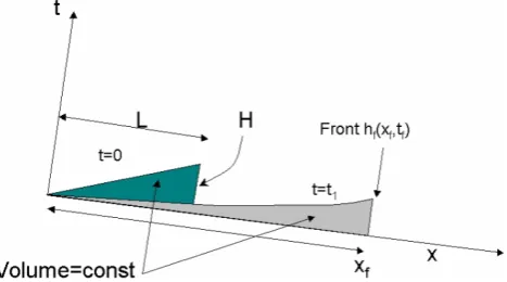
One of the assumptions made by the authors is that the total volume of the debris flow remains constant during the entire propagation process, that is no erosions or depositions take place or erosions and depositions balance out (Arattano and Savage, 1994). At timet=0, the shape of the debris flow is assumed to be triangular, with a total lengthL and front depthH(Fig. 1), according to:
(
0≤x≤L h=bHLx for t
=0 (7)
M. Arattano and L. Franzi: On the application of kinematic models 1691
Fig. 1. Scheme of kinematic wave, as proposed by Arattano and
Savage (1994).
(assuming a rectangular shape of the channel):
b
xf
Z
0
hdx=bLH
2 (8)
Integration of Eq. (8) starts atx=0 and stops atx=xfwhere the integral is equal to the total volume. Since the starting point of the integration remains fixed (x=0), the integration is implicitly carried out assuming that, for any given ε>0 arbitrarily chosen:
ε
Z
0
hdx >0 (9)
As a consequence of the assumption of a constant volume and of the integration over the intervalx=[0;xf], the front height must progressively decrease. This is a result of the particular choice of the boundary conditions needed to solve the system equations given by Eq. (1) and Eq. (3). This can be easily understood if we consider that the portion of the wave behind the peak, that is the decreasing limb of the hy-drograph, follows the peak with a slower velocity. This is due to the direct dependency of velocity on flow height, as expressed by Eq. (3), and to the progressive decrease of flow height behind the main wave front due to the assumption of a triangular form for the initial debris mass. Thus, the whole debris flow wave elongates and the continuity equation then imposes the peak height to decrease.
It must be noticed that a different choice of the boundary conditions would have lead to completely different results. As a matter of fact, very different boundary conditions can be imposed for a kinematic model and these can then greatly influence the final results. As an extreme example, it could even be possible to impose that the integration starts from the front that flows downstream with a celerity given by:
c=ks(n+1)Hn
√
S (10)
These choices correspond in adopting an integration interval
16 1
Figure 2. Scheme of kinematic wave, as proposed by Eq(s).(12 - 13). 2
3
Fig. 2. Scheme of kinematic wave, as proposed by Eqs. (12–13).
that ranges between the front itselfxfand the position of the tail. In this way, the integral (8) becomes:
x(h=H )
Z
xt
bhdx=bLH
2 (11)
wherex(h=H )is the abscissa where the debris flow height ish=H, andxt is the tail of the debris flow, where the flow depth is not necessarily equal to zero.
Even though this would lead to unrealistic results, it could nevertheless be mathematically imposed and the equation could be consequently solved to obtain:
xf=L+ks(n+1)Hnt
√
S (12)
ksnHn+1
√
St−ksn(htail)n+1
√
St−L
H h2tail
2 =0 (13)
These equations predict that the tail thickens downstream and that the head of the debris flow remains unchanged (Fig. 2). Note that the latter is a consequence of the particular choice of the integration interval and it is not imposed a-priori.
As mentioned earlier, these results are unrealistic but they are presented here to show the strong dependency of the solu-tion on the specific boundary condisolu-tions that are chosen. The capability of the Arattano and Savage (1994) model to sim-ulate debris flow propagation and the diffusive effects that take place in nature only derives from a peculiar choice of the boundary conditions, while the model still remains inca-pable of simulating the natural diffusions taking place along the debris flow wave.
Fig. 3. The Moscardo Torrent basin (3) and its alluvial fan (4). (1)
Debris flow initiation area; (2) instrumented channel stretch where two ultrasonic sensors are placed 75 m apart from each other.
that took place in Rio Moscardo (North-Western Italy, Fig. 3) on 23 July 2004, and to compare the respective roles played by the diffusion and by the kinematic terms. A detailed de-scription of the debris flow that has been simulated can be found in Arattano et al. (2006). In the following figure, a sketch of the instrumented watershed basin is shown, with the location of the ultrasonic gauges.
The debris flow stage was measured by two ultrasonic gauges, at two different cross-sections. The lymnographs al-lowed us to investigate on the rheology of the recorded de-bris flow (Arattano at al., 2006) by means of a mathematical model. In the latter, the upstream hydrograph (Fig. 4) was used to set the upstream boundary conditions.
The simulated results have been compared to the flow heights recorded at the downstream cross-section by the sec-ond ultrasonic sensor.
3 Kinematic-diffusive model
As previously mentioned, Eq. (3), which is a simplified form of the Saint-Venant momentum equation, implies that no physical diffusion is taken into account in the simulations, since diffusion is a second-order effect. However, physical diffusion cannot be neglected a priori. In fact, along the in-creasing limb of the hydrograph in particular, the depth
gra-18 0
0.5 1 1.5 2 2.5
0 100 200 300 400 500 600 700 800 time (s)
d
e
p
th
(
m
)
Recorded 2
3
Figure 4. Upstream lymnograph of the debris flow occurred on July 23, 2004 4
5
6
Fig. 4. Upstream lymnograph of the debris flow occurred on 23 July
2004.
dient is no more negligible and, as a consequence, Eq. (3) does not hold any more. The discharge is higher than that cal-culated with Eq. (3) along the rising limb of the hydrograph, and it is smaller along its falling limb, as it is expressed by the so-called looped stage-discharge curves (Chow, 1959).
Lighthill and Witham (1955), in order to take into account a small amount of diffusion, tried to extend the kinematic model by considering the terms that depend on the flow gra-dient and neglecting the momentum source terms and the terms that depend on local inertia.
By considering the continuity equation and the momentum equation together (where the local inertial and convective in-ertial terms are neglected), it is obtained (Ponce, 1991, 1992; Todini, 2007):
1
c ∂Q
∂t +
∂Q
∂x −υ
∂2Q
∂x2 =0 (14)
withc andυ that are the kinematic wave celerity and hy-draulic diffusivity, respectively, defined as:
c=1
b dQ
dh (15)
υ= Q
2bS0
(16) Equation (14) can be solved either analytically or numeri-cally.
In the present work, a nonlinear model recently proposed by Todini (2007), for the computation ofQ(candυ vary with time) will be used to compare the roles played by the diffusion terms and by the kinematic terms.
The computation ofh, can be made by solving the continu-ity equation, Eq. (1), by means of a first order approximation:
1
b α
Qni −Qni−1
1x +(1−α)
Qni+1−Qni−+11 1x
!
+ βh
n+1 i −h
n i
1t +(1−β)
hni−+11−hni−1 1t
!
M. Arattano and L. Franzi: On the application of kinematic models 1693
Q(xi,tn);h(xi,tn), withxi=x0+i1x;tn=t0+n1t, being
i=1,2,...,M;n=1,2,...,N, andα,β numerical parame-ters of integration (Abbot and Cunge, 1982).
The model givesQ=Q(c,υ), where both celeritycand diffusivityυ depend on the Courant number Cn, defined as follows (Todini, 2007):
Cn= wave.celerity
computation.celerity (18)
The model allows the computation of the total height of the debris flow in space and time, it is mass conservative, and al-lows the comparison of the role played by the diffusion terms in Eq. (14) and that played by kinematic terms.
4 Application of the kinematic-diffusive model
Todini’s (2007) diffusive model was applied to simulate the propagation of a debris flow which occurred on 23 July 2004 in the Moscardo torrent, an instrumented basin located on the northeastern Italian Alps (Fig. 3) (Arattano et al., 1997).
The debris flow depths were measured at two different cross-sections, located 75 m apart, by means of two ultra-sonic sensors. The availability of two hydrographs (Figs. 4 and 5) has allowed the calibration of the rheological param-eters of Eq. (3) (Arattano et al., 2006). The upstream hy-drograph has been used as an upstream boundary condition, while the downstream hydrograph has been used to compare the simulation results and the recorded data.
The values of the rheological parameters of Eq. (3) have been assumed to be the same as those obtained by Arattano et al. (2006), employing the complete Saint-Venant equations, namelyks=4 m−0.8/s andn=1.2. The results (Fig. 5) show a good match between computed and recorded hydrographs.
Note that the passage of the debris flow has increased the bed elevation at the downstream station. This could be due to the filling of some erosion under the downstream ultrasonic sensor that took place before the arrival of the debris flow. Thus, the bed elevation surveyed after the passage of the de-bris flow has been used in the simulation and this explains the significantly different flow stage that the simulation and the recordings show in Fig. 5 before the arrival of the debris flow front.
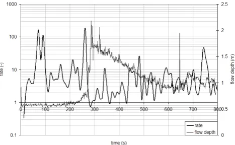
The goal of evaluating the amount of physical diffusion in the recorded debris flow has been pursued calculating the ratio:
rate=
1 c
∂Q ∂t +
∂Q ∂x
υ∂2Q
∂x2
(19)
This ratio compares the sum of the first and second terms of Eq. (14) to the third one. It is noticeable that if in Eq. (14) one assumesυ=0, the model expressed only by the sum of the first and second term, that is:
1
c ∂Q
∂t +
∂Q
∂x =0 (20)
Fig. 5. Comparison of recorded and simulated hydrograph
(simula-tion performed with1x=1 m;1t=1 s) at the downstream reach.
Fig. 6. Rate given by Eq. (19).
is the same as the kinematic model. Consequently the higher the rate given by Eq. (19), the higher the influence of kine-matic terms is, with respect to the diffusive term (second par-tial derivative).
In Fig. 6, a plot with the value of this rate for the down-stream hydrograph is shown. Figure 6 shows that the dif-fusion term can be of the same order of magnitude as the remaining terms. This means that diffusive effects cannot be neglected a priori. Their main effects are exerted in the front of the debris flow, where the curvature ofQis also not negligible. Therefore, the application prefers a mathematical model capable of taking into account the diffusion terms.
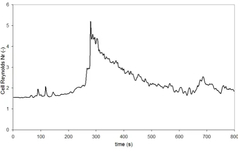
Fig. 7. Rate of the physical diffusivity to numerical diffusivity
(Eq. 21).
Since Todini’s (2007) model is applied through a numeri-cal simulation, it has inevitably introduced some amount of numerical diffusion. In order to compare the effects due to numerical and physical diffusion, it is possible to use the cell Reynolds number,D, introduced by Todini (2007).
Dis given by the ratio between the physical and numerical diffusivity, that is:
D= Q
bS0c1x
(21) The largerDis, the higher is the role of the physical diffu-sivity.
In the simulated debris flow (Fig. 7)D is always larger than 1, with a maximum of 5 in the proximity of the front of the debris flow. This confirms that, assuming 1x=1 m and1t=1 s, the physical diffusivity prevails on the numerical one.
Thus, a numerical model can be safely employed without greatly affecting the results because of the numerical dissi-pation.
5 Conclusions
The diffusive processes that take place in debris flow can be mathematically simulated only if second order terms are taken into account in the Saint-Venant equation. Conse-quently kinematic models, though widely used in the litera-ture, cannot fairly reproduce the dissipation that take place in real debris flows. However, due to a particular choice of boundary conditions, it has been shown that a kinematic model expressed in analytical form allows the simulating of two large-scale diffusion effects: the downstream spreading of the debris-flow wave and the progressive decrease of its main front height. Then a mathematical convective-diffusive model has been used to simulate a field debris flow which occurred in 2004 in an Italian torrent, whose rheological be-haviour has been described by means of a Ch´ezy-like
for-mula. The effects of local diffusion have been determined and compared with the effects due to other terms. Physical diffusive processes and processes due to numerical diffusion have also been quantified and compared. The results showed that physical diffusion processes are not negligible with re-spect to kinematic (mass transfer) processes. Therefore, the application of a mathematical model capable of taking into account the diffusion terms should be preferable and it has been shown that a numerical model can be safely employed without greatly affecting the results because of the numerical dissipation that it inevitably introduces.
Appendix A
List of symbols (SI units).
b = width of the flow
c = kinematic celerity
Cn = Courant number (dimensionless)
D = cell Reynolds number (dimensionless)
h = flow depth
H = initial height of the debris flow front
hf = height of the front of the debris flow
htail = height of the tail of the debris flow
ks,n = rheological parameters
L = initial length of the debris flow
M = total number of space steps of integration
N = total number of time steps of integration
Q = total discharge (water and sediment)
S = energy gradient (dimensionless)
S0 = channel bottom slope (dimensionless)
t0 = time at whichhfis at thexfprogressive
U = mean velocity of the flow
x,t = independent variables (time and space)
xf = abscissa of the front of the debris flow
xt = abscissa of the tail of the debris flow
1x,1t = finite differences inxandt
α,β = numerical parameters (dimensionless)
υ = hydraulic diffusivity
Acknowledgements. The researches on debris flows in the
Moscardo Torrent were initiated by M. Govi and carried out during the years by several researchers and technicians of CNR IRPI, in particular L. Marchi. We also thank the Forest Department of Friuli-Venezia Giulia Region for their collaboration in installing and managing field instrumentation.
Edited by: M. Arai
M. Arattano and L. Franzi: On the application of kinematic models 1695 References
Abbott, M. B. and Cunge, J. A.: Engineering Application of Com-putational Hydraulics, Pitman Books Limited, 1982.
Arattano, M., Franzi, L., and Marchi, L.: Influence of rheology on debris-flow simulation, Nat. Hazards Earth Syst. Sci., 6, 519– 528, doi:10.5194/nhess-6-519-2006, 2006.
Arattano, M., Deganutti, A. M., and Marchi, L.: Debris flow moni-toring activities in an instrumented watershed on the Italian alps, in: Proceedings of the First International ASCE Conference on Debris-Flow Hazard Mitigation: Mechanics, Prediction and As-sessment, San Francisco, Ca, 506–515, 7–9 August 1997 Arattano, M. and Marchi, L.: Systems and sensors for debris-flow
monitoring and warning, Sensors, 8, 2436–2452, 2008. Arattano, M. and Savage, W. Z.: Modelling debris flows as
kine-matic waves, Bull. Int. Assoc. Eng. Geol., 49, 95–105, 1994. Chow, V. T.: Open channel hydraulics, McGraw-Hill, Tokyo, 1959. Genevois, R., Tecca, P. R., Berti, M., and Simoni, A.: Debris flows in the dolomites: experimental data from a monitoring system, in: Proceedings of the 2nd International conference on debris flows hazard mitigation: mechanics, prediction and assessment, Taipei, Taiwan, 283–29, 16–18 August 2000.
H¨urlimann, M., Rickenmann, D., and Graf, C.: Field and monitor-ing data of debris-flow events in the Swiss Alps, Can. Geotech. J., 40(1), 161–175, 2003.
Iverson, R. M.: The Physics of Debris Flows, Rev. Geophys., 35(3), 245–296, 1997.
Johnson, A. M.: Physical processes in Geology, Freeman, Cooper and Co, 1970.
Lanzoni, S. and Tubino, M.: Rheometric experiments on mature de-bris flows, in: Proceeding of the 25th I.A.H.R. congress, Tokyo, Japan, 47–54, 30 August–3 September 1993.
Lighthill, M. J. and Whitham, G. B.: On kinematic waves, in: Flood movement in long rivers, P. R. Soc. Lond. A, Piccadilly, London, 281–316, 10 May 1955.
Pierson, T. C.: Flow behaviour of channelized debris flows, Mount S. Helens, Washington, in: Hillslope processes, edited by: Abra-ham, A. D., Allen & Unwin, Boston, 269–296, 1986.
Pierson, T. C., Janda, R. J., Thouret, J. C., and Borrero, C. A.: Per-turbation and Melting of Snow and Ice by the 13 November 1985 Eruption of Nevado del Ruiz, Colombia, and Consequent Mo-bilization, Flow and Deposition of Lahars, J. Vulcanol. Geoth. Res., 41, 17–66, 1990.
Ponce, V. M.: Kinematic Wave Modelling Where Do We Go From Here?, in: Proceedings of the International Symposium on Hy-drology of mountainous areas, Shimla, India, 485–495, 28– 30 May 1992.
Ponce, V. M.: The kinematic wave controversy, J. Hydraul. Eng.-ASCE, 117(4), 511–525, 1991.
Pudasaini, S. P., Wang, Y., and Hutter, K.: Modelling debris flows down general channels, Nat. Hazards Earth Syst. Sci., 5, 799– 819, doi:10.5194/nhess-5-799-2005, 2005.
Takahashi, T.: Debris flows, Balkema, Rotterdam, 1991.