Prediction Of Fagm(1,1) Model Based On Cotes Formula In China's Local Fiscal Expenditure

(1)

Vol. 5 Issue 1, January - 2019

Prediction of FAGM(1,1) Model Based on

Cotes Formula in China's Local Fiscal

Expenditure

Lang Yu1*

Southwest University of Science and Technology School of Science

Mianyang, China [email protected]

Xiwang Xiang2

Southwest University of Science and Technology School of Science

Mianyang, China

Abstract—In this paper, the fractional-order CFAGM (1,1) grey prediction model improved by the Cotes integral formula is established and the local fiscal expenditure in China is predicted. First, a fractional-order FAGM(1,1) model is established based on the fractional-order

accumulation generation operator and the

fractional-order accumulation generation

operator. Secondly, the Cotes integral formula is used to improve the background value of the FAGM(1,1) model, and the CFAGM(1,1) model is established. Further, the GM(1,1) model, the FAGM(1,1) model and the CFAGM(1,1) model are compared and analyzed. It can be clearly seen that the CFAGM(1,1) model is more than GM(1,1). And the FAGM (1,1) model has higher prediction accuracy in the prediction of local fiscal expenditure.

Keywords—local fiscal expenditure; fractional grey prediction model; Cotes formula

I. INTRODUCTION (Heading 1)

Fiscal expenditure is an important part of the fiscal system and has an irreplaceable position in the implementation of national fiscal policy and economic development. It can fully reflect the total amount of economic activity and measure the level of development of a region or national economy. China's fiscal expenditure is divided into local fiscal expenditure and central government expenditure. Compared with the regulation of central government expenditures, regulating local fiscal expenditures will have more direct or indirect effects on people's lives.

Therefore, accurately predicting local fiscal

expenditure has very important practical and practical effects on the macroeconomic regulation and control of the local economy and the preparation of local financial budget reports. At present, the main prediction methods at home and abroad include: trend extrapolation method, exponential smoothing method, time series method, fuzzy prediction method, regression analysis method and other prediction

methods. But these methods have certain

requirements for the data. It can be seen that the prediction of local fiscal expenditure is a long-term, complex, but significant practical work.

There have been a lot of research results on the prediction of fiscal expenditure. Chen et al. [1]

introduced the autoregressive single-moving average model to predict and analyze fiscal expenditures; Sun et al. [2] used time-series data VAR model to predict the trend of China's fiscal expenditure scale change; Zhang [3] The ARMA model is applied to the analysis and prediction of China's fiscal expenditure, and is implemented by SAS; Jing et al. [4] use VAR model to dynamically predict and structure local fiscal revenue; He [5] and others use The GM(1,1) model models and predicts the local fiscal revenue and expenditure of Xianning City; Hu [6] conducts the time-sequence ARMA model of China's fiscal technology expenditure value to carry out the scientific and technological expenditure value of China's "Twelfth Five-Year Plan" period. Predictive research; Ren [7] used the ARIMA model to conduct short-term forecast analysis of Henan Province's fiscal expenditure data; Mei [8] used the intervention analysis method proposed by Box and Tiao to intervene in fiscal expenditure forecasting. The analysis is carried out; Chen [9] discusses the forecasting model and control model of fiscal revenue and expenditure using the principles and methods of optimal cybernetics; Wang [10] Research on the Chinese to predict the scale of expenditure by the base method. From the above research results, the models for fiscal expenditure forecasting mainly include time series model, gray GM (1, 1) model, autoregressive model and cardinal method. The time series method is based on the historical data of fiscal expenditure. The method is simple to calculate, but it is difficult to reflect the internal laws of the data. The gray GM (1,1) model requires less modeling data and less calculation. The data is required to have the characteristics of exponential growth; the cardinal method is subject to intervention by human factors, and the consideration is single, so that the budget arrangement cannot be synchronized with the actual dynamic management.

(2)

economy [24-27] and other aspects of society. However, the classic GM (1,1) model has some shortcomings, such as the first degree of accumulation of the original data, making the model less flexible. Therefore, Wu [28-32] first proposed a fractional gray model, and analyzed its properties in detail, and gave specific numerical examples. The results show that the fractional gray prediction model has better prediction effect than the classical GM (1,1) model. As a result, many experts and scholars have emerged theoretically and improved research on fractional grey theory.

Based on the above research, this paper proposes a fractional accumulation order CFAGM(1,1) model based on the Cotes formula, and uses this model to model and predict local fiscal expenditures in China. The local fiscal expenditure data of China Statistical Yearbook [33] 2001-2007 is used as model fitting data, and the data from 2008-2012 is used as extrapolation forecast data to test the prediction accuracy of the model. The prediction results of the classical GM (1,1) model, FAGM (1,1) model and CFAGM (1,1) model are compared and analyzed. The results show that the fractional accumulation order CFAGM(1,1) model improved based on the Cotes formula has better prediction accuracy.

II. PREREQUISITE KNOWLEDGE

A. Accumulator operator

Definition Original non-negative sequence  0



 0

_{ }

 0

_{ }

 0

_{ }

 0

_

_

 0

_{ }



1 , 2 , 3 1 ,

X  x x x x n x n ,the

r-order accumulation generation sequence

(

rAGO

)

is:

 



 

_{ }

 

_{ }

 

_{ }

 

_

_

 

_{ }



1 , 2 , 3 1 , .

r r r r r r

X  x x x x n x n (1)

Among them:

 

_{ }







  

 0

 

1

, 1, 2,3, , . 1

k r

i

r k i

x k x i k n

k i r



  

 

   



(2)







  







 









 



1 2 1

1 1 !

1 !

, 1, 2, 3, , .

! 1 !

r k i k i k i k i r

k i r r

r k i

k n

k i r

         



    

  

 

 

(3)

The r-order accumulation generation sequence matrix is expressed as:

   0

.

r r

X X X (4)

Among them:  

                   

              

       

     

1 2 1

1 2 3

1 2

0

1 2 1

. 3

0 0

1 2

0 0 0 0

1

r

r r r r n

r r r n r

r r r n

r r n r

X r r n

r n r

r r

       

 

_ _ _ _ _ _ _ _ 

 

 _ _{ } _{  } 

 

      

 

_     _

 _ _ _{  } 

 

 _ 

 

   

 

(5)

 1



 1

_{ }

 1

_{ }

 1

_{ }

 1

_

_

 1

_{ }



1 , 2 , 3 1 , .

X  x x x x n x n

₍₆₎

B. Reducing operator

Definition Set the original non-negative sequence

 0



 0

_{ }

 0

_{ }

 0

_{ }

 0

_

_

 0

_{ }



1 , 2 , 3 1 ,

X  x x x x n x n ,the r-th

order subtraction generation sequence rIAGO is:

 r



 r_{ }_{1 ,}  r _{ }_{2 ,}  r _{ }₃  r_ _{1 ,}_  r _{ }



_.

X  x x x x n x n ₍₇₎

Among them:

 _{ } _{ }  

      

1

0 0

1

1 , 1, 2,3, , .

1 1

k i r

i

r

x k x k i k n

i r i

 



 

   

    



(8)

In particular, the operator 1IAGO is generated for the first-order subtraction when

r



1 .

 1



 1

_{ }

 1

_{ }

 1

_{ }

 1

_

_

 1

_{ }



1 , 2 , 3 1 , .

X  x x x x n x n (9)

C. Cubic spline interpolation

In many engineering calculation problems, there is a high requirement for the smoothness of the

interpolation function. Although the high-order

polynomial interpolation has higher smoothness, the calculation amount is large, the error is large, and sometimes the Rung phenomenon occurs; the low-order segmentation interpolation although the Rung phenomenon can be avoided and the calculation is simple, the inserted function can be well approximated, but the smoothness is poor. Thus, a spline interpolation method is produced. The so-called spline interpolation, this is an early engineer when drawing graphics, using flexible fine wood strips or thin metal strips (splines) to connect some known points into a smooth curve, and make known points There is a continuous second derivative, which abstracts the cubic spline interpolation function.

Definition If function

S x

 



C

2

 

a b

,

and

0 1 1

:

_n _n

T a



x

 

x



x

_



x



b

is a division of

interval

[a, b]

，That is,

x i

_i

,



0,1, 2,

,

n

is a known node. If on each subinterval



x

i₁

,

x

i



,

i



0,1, 2,

,

n

，

S x

 

is a cubic polynomial，and

S x

 

has a 2nd

order continuous derivative on

[a, b]

，Then

S x

 

is

called the cubic spline function for dividing

T

.

If function

y



f x

 

has a function value of n+1 known nodes on interval

[a, b]

:

 

, 0,1, 2,3, , .

i i i

y  f x S x i n (10)

Then

S x

 

is called cubic spline interpolation

(3)

Vol. 5 Issue 1, January - 2019 III. FRACTIONAL ORDER ACCUMULATION FAGM (1,1)

MODEL

DefinitionLet

 0



 0

_{ }

 0

_{ }

 0

_{ }

 0

_

_

 0

_{ }



1 , 2 , 3 1 ,

X  x x x x n x n

be the

original sequence,

 r



 r

_{ }

_{1 ,}  r

_{ }

_{2 ,}  r

_{ }

₃  r

_

_{1 ,}

_

 r

_{ }



X  x x x x n x n ,X r is the

r-order accumulation sequence of  0

X ,(rIAGO). Let  r



 r

_{ }

_{2 ,}  r

_{ }

_{3 ,} _,  r

_{ }



Z  z z z n be the sequence of the

nearest mean (the background value) of X r

.

Among them:

 

_{ }

 



1



, 2, 3, , . 2

r r

r x k x k

z k    k n (11)

Known as the gray differential equation:

 

_

_

 

_{ }

 

_{ }

1 .

r r r

x k x k az k b (12)

This is an r-order accumulation gray GM (1,1) model.

Particularly, when r1,

 

_

_

 

_{ }

 

_{ }

1

r r r

x k x k az k b

becomes

x

 0

 

k



az

 1

 

k



b

, That is, the mean

GM (1, 1) model.Among them:

 

_{ }







  

 0

 

1

, 1, 2,3, , . 1

k r

i

r k i

x k x i k n

k i r



  

 

   



.

a

is the

coefficient of development,

b

is made of gray dosage. Model parameters can be solved by least squares. Set

the parameter to

u

ˆ



 

a b

,

T , Obtained by least squares method:

 

1

ˆ T T .

u B B  B Y (13)

Among them:

 _{ }

2 1 2 1

2 1 r r

r

z

z B

z

 

 



 

  

 

_ 

 

,

 

_{ }

 

_{ }

 

_{ }

 

_{ }

 

_{ }

 

_

_

2 1

3 2

. 1

r r

x x

Y

x n x n

  

 



 

  

 

 _ _ 

 

(14)

Definition. Set the model parameters as defined above, then

 

_{ }

 

_{ }

r

dx t

ax t b

dt   (15)

It is the whitening differential equation of the r-order accumulation gray GM(1,1) model.To solve equation (13), assume _ˆ 0

 

 0

 

1 1

x x , the time response

sequence is:

 

_{ }

 0

_{ }

 1

ˆr 1 b a k b, 2,3, , 1, .

x k x e k n n

a a

 

 

_  _   

  (16)

Thus, the resulting reduction value is:

 _{ }

 

  _{ } _{ }  

     

1 0

0

1

ˆ ˆ 1 ˆ , 2,3, , .

1 1

k

r i

r r

i

r

x k x k x k i k n

i r i

 



 

    

    

 (17)

Among them:  



r 1



r!,       



i 1



i!,



r i 1

 

r i



.

IV. FRACTIONAL ORDER ACACCUMULATION CFAGM

(1,1) MODLE

A. Error Analysis of Traditional GM(1,1) Model

From the original FAGM (1,1) reduction time response sequence, the accuracy of the FAGM(1,1) prediction model depends on the parameters

a

,

b

.

However, it is determined that the parameters

a

and

b

are

z

 r

( )

k

.

Therefore, the FAGM(1,1) model error

mainly comes from the calculation of

z

 r

( )

k

.Integrate

 

_{ }

 

_{ }

r

dx t

ax t b

dt  

on [k1, ]k ,so:    

1 (t) 1 ( ) 1 , 2,3,..., 1.

k _r k _r k

k k k

I dx a x t dt b dt k n

  



_



_



_

  (18)

Formula (18) combined with

 

_

_

 

_{ }

 

_{ }

1

r r r

x k x k az k b,therefore.

   

_{ }

1

( ) k .

r r

k

z k x t dt





_

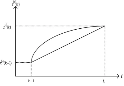
(19)

The geometric meaning of the background value of the FAGM(1,1) model is shown in the figure below. It can be clearly seen that the area of the curved trapezoid surrounded by the curve  r

 

x t in the

interval [k1, ]k and the horizontal axis

t

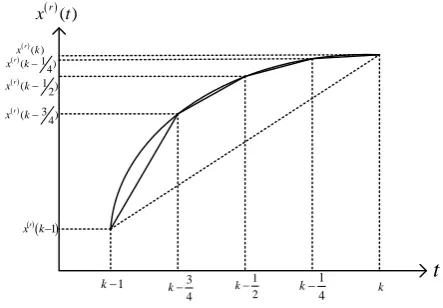
is the background value of the FAGM (1,1) model. The traditional way of calculating is to calculate the area of the trapezoid. As shown in Fig 1. Using the numerical integral Cotes formula (Newton-Cotes formula for n=4), the background value of the FAGM(1,1) model is the area of the curved trapezoid on the interval. As shown in Fig 2. It can be seen that the error generated by its calculation is significantly smaller than the traditional calculation method.

 

( )

r

x t

 

( ) r

x k

 

( 1) r

x k

1

k _k

t

(4)

Vol. 5 Issue 1, January - 2019   ( ) r x t 1

k k

t

3

4

k 1

4

k

1 2 k

 r_{( )}

x k

 r( 1₄) x k

  ₁

( ₂)

r

x k

 ( 3 ) 4

r

x k

 _{ }

1

r

x k

Fig 2. Cotes formula calculates the background value

B. Improved fractional CFAGM(1,1) model of Cotes

formula

Consider the integral of (19) on the interval

[k1, ]k , Using the Cotes formula in the numerical integration formula, Insert three equal points into the r-order accumulation sequence interval [k1, ]k and divide the interval [k1, ]k into quarters. Since the statistical observation data are some discrete data points, they are still discrete points after the r-th order accumulation. Therefore, this paper uses cubic spline interpolation to perform function approximation to supplement the function values of other insertion points in interval [k1, ]k .The integration interval is

[k1, ]k , Divide the interval [k1, ]k into 4 parts, Each node is recorded as:

1 1

, 2,3,..., .

4 4

k k

h   = k n

   

_

_

1 , ( 0,1, 2,3, 4).

k

r r

i

x x k ih i

(20)

Then consider the integral of (19) on

[

k



1, ]

k

,

   

2 2

1 (t) 1 ( ) 1 , 2, 3,..., .

k _r k _r k

k k k

I dx a x t dt b dt k n

  



_



_



_

 (21)

Equation (21) can be further expressed as:

     

2 2

1

( ) ( 1) k ( ) , 2,3,..., .

r r r

k

Ix k x k a



_x t dtb k n (22)

Combine the cubic spline interpolation function, Usingthe Cotes integral formula, Calculate the integral

of  

1 ( )

k _r

k x t dt



on [k1, ]k ,can be drawn

           

1 0 1 2 3 4

1

( ) 7 32 12 32 7

90

2,3,..., .

k k k k k

k _r _r _r _r _r _r

k

I x t dt x x x x x

k n

  

  _     _

 



₍₂₃₎

Then (21) can be expressed as:

     

           

1 1 2

0 1 2 3 4 2

( ) ( 1) ( )

( ) 7 32 12 32 7

90

2, 3,..., .

k k k k k

k

r r r

k

r r r r r r

I x k x k a x t dt

a

x k x x x x x b

k n           _     _ 



(24)

Compare the background value of (19) with

z

 r

( )

k

:

 _{ }          

0 1 2 3 4

1

7 32 12 32 7 2, 3,..., .

90 k k k k k

r r r r r r

z k  _ x  x  x  x  x _，k n ₍₂₅₎

Further simplification (24) has:

 1          

90 r ( ) 7 r 32 r 12 r 32 r 7 r 90 0

x  k a  x  x  x  x  x  b 

Remember that





2 2, 2 T

u  a b is a constant column,

which is known by the principle of least squares. The parameter column needs to satisfy:

1

2 2 2 2 2

ˆ ( T ) T .

u  B B  B Y (27)

Among them:

         

2 2 2 2 2

3 3 3 3 3

0 1 2 3 4

2

0 1 2 3 4

1

7 32 12 32 7 1

90 1

7 32 12 32 7 1

, 90

1

7 32 12 32 7 1

90 n n n n n

r r r r r

x x x x x

B

x x x x x

_ _ _ _ _ _ _        _ _ _ _ _ _ _            _ _        _ _     _{ }  _{ }  _{ }  _{ }  _{ }  _ _ 2 2 1 3 2 . 1 r r r r r r x x x x Y

x n x n

              _ _    (28)

C. Model test

The error of the model is an important indicator for evaluating the reliability and practicability of a model. In this paper, in order to verify the prediction accuracy

of the model, The mean square error (MSEOTFE) of

the fitted data is calculated mainly based on the predicted value and the actual value. The average relative error of extrapolated predicted values (

AREOPV ).And the total mean relative error (TARE) to represent the error of the model. Its calculation formula is as follows:

 _{ }  _{ }





2

0 0 1 1 ˆ . N k

MSEOTFE x k x k

N 





 ₍₂₇₎

 _{ }  _{ }  _{ } 0 0 0 1 ˆ 1 . n k N

x k x k

AREOPV

n N   x k

 





(28)

 _{ }  _{ }  _{ } 0 0 0 1 ˆ 1 . n k

x k x k

TARE

n  x k







₍₂₉₎

Where

n

is the number of total sample data and

N

is the number of data used to fit the model. Obviously,

the smaller

MSEOTFE

,

AREOPV

and

TARE

, the

better the prediction of the model. Case Analysis

V. CASE ANALYSIS

In order to verify the practicality and effectiveness of the above improved model CFAGM(1,1), This paper obtains the local fiscal expenditure from 2001 to 2012 from the China Statistical Yearbook as empirical analysis data. The data from 2001-2007 was used as the model fitting data, and the data from 2008-2012 was used as the forecasting data. The local fiscal expenditure data for 2001-2007 is shown in the following Table 1:

Table 1. Statistics of local fiscal expenditures from 2001 to 2007.(Unit: 100 million yuan)

Year 2001 2002 2003 2004 2005 2006 2007 Local

(5)

For comparison, the GM(1,1) model, FAGM(1,1) model and CFAGM(1,1) model are established respectively. Using the above Table 1 data for modeling and fitting, the optimal order of the FAGM(1,1) model and the

CFAGM(1,1) model were calculated by MATLAB

software to be -0.06 and 1.28, and predicted 5 years later. The fitting results and prediction accuracy were compared and analyzed. The fitting results of the three

models are shown in Table 2 below:

Table 2: Comparison of the fits of different model (Unit: 100 million yuan) Years Actual

value GM(1,1)

Relative

error./% FAGM(1,1)

Relative

error./% CFAGM(1,1)

Relative error./% 2001 13134.56 13134.56 0.00 13134.56 0.00 13134.56 0.00 2002 15281.45 14179.94 -7.21 15283.73 0.01 15377.58 0.63 2003 17229.85 17206.81 -0.13 17675.22 2.58 17193.92 -0.21 2004 20592.81 20879.79 1.39 20749.24 0.76 20500.84 -0.45 2005 25154.31 25336.81 0.73 24873.04 -1.12 24995.73 -0.63 2006 30431.33 30745.23 1.03 30501.70 0.23 30802.90 1.22 2007 38339.29 37308.13 -2.69 38247.49 -0.24 38180.54 -0.41

MSEOTFE 2491327 315319.9 207407.8

Fig 3 Comparison of fitting and prediction results based on different models

It can be seen from Table 2 that the

MSEOTFE

of the CFAGM(1,1) model is 207407.8, while the

MSEOTFE

of the GM(1,1) model and the

FAGM(1,1) model are 2491327 and 315319.9, respectively, both higher than CFAGM(1,1). model. It can be seen from Fig.3 that the improved CFAGM(1,1) model has higher prediction accuracy than the GM(1,1) model and the FAGM(1,1) model. It can be seen that the improved CFAGM(1,1) model has better fitting effect and prediction accuracy than the GM(1,1) and FAGM(1,1) models. Table 3 below shows the extrapolated predictions for different models.

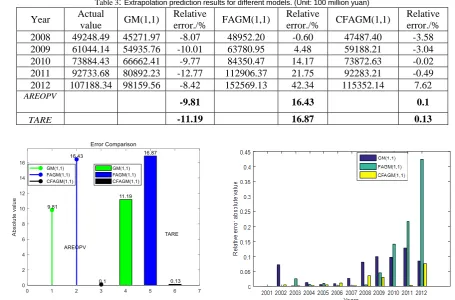
Table 3: Extrapolation prediction results for different models. (Unit: 100 million yuan) Year Actual

value GM(1,1)

Relative

error./% FAGM(1,1)

Relative

error./% CFAGM(1,1)

Relative error./% 2008 49248.49 45271.97 -8.07 48952.20 -0.60 47487.40 -3.58 2009 61044.14 54935.76 -10.01 63780.95 4.48 59188.21 -3.04 2010 73884.43 66662.41 -9.77 84350.47 14.17 73872.63 -0.02 2011 92733.68 80892.23 -12.77 112906.37 21.75 92283.21 -0.49 2012 107188.34 98159.56 -8.42 152569.13 42.34 115352.14 7.62

AREOPV

-9.81 16.43 0.1

TARE -11.19 16.87 0.13

(6)

From the above Table 3 and Fig 4 (left), the

AREOPV of the GM(1,1) model, the FAGM(1,1)

model and the CFAGM(1,1) model are respectively -9.81%, 16.43%, 0.1%；Their TARE are respectively -11.19%, 16.87%, and 0.13%, among them, the

AREOPV and

TARE

of the CFAGM (1,1) model are smaller than the other two models.

VI. CONCLUSION

This paper proposes a fractional-order CFAGM(1,1) model based on the Cotes integral formula, which is compared with the classical GM(1,1) model and FAGM(1,1) model by theoretical derivation and examples. In the analysis, the fitting effect and prediction effect are better than the GM(1,1) and FAGM(1,1) models. Secondly, the CFAGM(1,1) model is smaller due to the improved calculation method of background values. The fitting error improves the prediction accuracy of the CFAGM(1,1) model. Finally, the prediction of the fractional-order CFAGM(1,1) model based on the Cotes formula proposed in this study is effective in predicting the local fiscal expenditure data in China. It validates the validity and practicability of the improved model, provides theoretical support for China's future macro-control of local fiscal expenditure, and prepares local financial budget reports. It also expands the application field of fractional-order prediction models. Both theoretical development and practical application have important values.

VII. REFERENCES

[1] Y.Chen, W.Zhao, X.T. Yan, Application of Autoregressive Single Moving Average Model in Financial Expenditure Forecasting[J]. Review of Economic Research,2014(33):53-62.

[2] C.Q. Sun , H. Li, W.T. Yu, Prediction of the Change Trend of Fiscal Expenditure Scale in China[J]. Sub National Fiscal Research, 2005(05): 46-49.

[3] S.Y. Zhang , Time Series Analysis of China's Financial Expenditure[J]. Journal of FuJian institute of education, 2009, 10(05): 43-46.

[4] H.J. Jing , L.C. Wang , Dynamic Prediction and Structural Analysis of Local Fiscal Revenue Based on VAR Model——Taking Heilongjiang Province as an

Example[J].Research of Finance and

Accounting,2015(03):5-9.

[5] G.S. He, R.G. Zhong, X.P. Zhou, L. Hu, Research on Financial Revenue and Expenditure Prediction and Operation Evaluation Based on GM(1,1) Model[J].Northern economy,2012(05):74-75.

[6] Z.F. Hu, Prediction analysis of national fiscal expendi ture on science and technology in China in the 12th five-year period based on ARMA model[J]. Science Mosaic,2013(05):211-213.

[8] Y. Mei, Intervention analysis in fiscal expenditure forecasting[J]. Inner Mongolia Financial Accounting, 1999 (12): 11-12.

[9] G.T. Chen, Forecast and control of regional revenue and expenditure[J]. Journal of Xiamen University(Natural Science), 1998(05): 26-29.

[10] J.P. Wang, 2050: Prediction of the Scale of China's Fiscal Expenditure[J]. Lanzhou Academic Journal, 2005(05): 116-117.

[11] J. L. Deng Contro1 problems of grey

systems[J]. Systems &Control Letters, 1982,

1(5):288_294.

[12] S.F. Liu,Y,G. Dang, Z.G. Fang, et al, Grey System Theory and Its Application [M]. Beijing: Science Press. 2010: 1-82.

[13] X.P. Xiao, S.H. Mao, Grey Prediction and Decision Method [M]. Beijing: Science Press. 2013:1-3.

[14] J.Wang ,R. Yan , K. Hollister , et al, A historic review of management science research in Сhіnа[J]. Оmеgа, 2008, Зб(б): 919-9З2.

[15]Y. Mu-shang , Fifteen years of grey system theory research: A historical review and

bibliometric analysis[J]. Expert Systems with Applications, 2013, 40(7): 2767-2775.

[16]U. Kumar,V.K. Jain, Time series models (Grey-Markov, Grey Model with rolling mechanism and singular spectrum analysis) to forecast energy consumption in India[J]. Energy, 2010, 35(4): 1709-1716.

[17] D.C. Li, C. J. Chang, C. C. Chen, et al, Forecasting short-term electricity consumpti on usingthe adaptive grey-based approach-An Asian case[J]. Omega, 2012, 40 (6):767-773.

[18]G.D. Li, S. Masuda, M. Nagai, The predi ction model for electrical power system using an improved hybrid optimization model[J]. Intemational Journa1 of Electrica1Power & Energy Systems, 2013, 44(1): 981-987.

[19]S.L. Ou, Forecasting agricultural output with an improved grey forecasting model based on the genetic algorithm[J]. Computers and Electronics in Agriculture, 2012, 85: 33-39.

[20]H.W.V. Tang, M.S. Yin, Forecasting

perfonmance of grey prediction for education expenditure and school enrollment[J]. Economics of Education Review, 2012,31(4):452-462.

[21] L.C. Hsu, C .H. Wang, Forecasting integrated circuit output using multivariate grey model and grey

relational analysis[J]. Expert Systems with

Applications, 2009,36 (2): 1403-1409.

(7)

[23]D. Golmohammadi, M. Mellat-Parast,

Developing a grey-based decision-making model for supplier selection[J]. Internati onal Journa1 of Production Economics, 2012,137(2):191-200.

[24]H.T. Pao, H.C. Fu, C.L. Tseng, Forecasting of CO2 emissions, energy consumption and economic growth in China using an improved grey model [J]. Energy,2012, 40(1):400-409.

[25]M.S. Yin, H.W.V. Tang, On the fit and forecasting performance of grey prediction models for

China's 1abor fomnation[J]. Mathematical and

Computer Modelling,2013,57(3-4): 357-365.

[26]T.S. Chang, C.Y. Ku, H.P. Fu, Grey theory analysis of online population and online game industry revenue in Taiwan[J]. Technological Forecasting & Social Change,2013,80(1): 175-185.

[27]S.J. Huang, N.H. Chiu, L.W. Chen, Integration of the grey relational analysis with genetic algonithm for software effort estimation[J]. European Journal of Operational Research,2008,188(3):898 -909.

[28] L.F. Wu, S.F. Liu, L.G. Yao, S.L.Yan, D.L. Liu, Grey system model with the fractional order accumulation, Communication in Nonlinear Science & Numerical Simulation, 2013, 18(7):1775-1785.

[29] L.F. Wu, S.F. Liu, W. Cui, D.L. Liu, T.X. Yao, Non-homogenous discrete grey model with

fractional-order accumulation, Neural Computing and

Applications, 2014, 25(5): 1215-1221.

[30] L.F. Wu, S.F. Liu, L.G. Yao, R.T. Xu, X.P. Lei, Using fractional order accumulation to reduce errors from inverse accumulated generating operator of grey model, Soft Computing, 2015,19(2): 483-488.

[31] L.F. Wu, S.F. Liu, Z.G. Fang, H.Y. Xu, Properties of the GM(1,1) with fractional order accumulation, Applied Mathematics and Computation, 2015, 252(1): 287-293.

[32] L.F. Wu, B. FU, GM (1,1) Model with fractional order opposite-direction accumulated generation and its properties[J]. Statistics & Decision, 2017, 18(5): 33-36.