http://theoryofcomputing.org
A Simple PromiseBQP-complete Matrix
Problem
Dominik Janzing
Pawel Wocjan
Received: October 22, 2006; published: March 30, 2007.
Abstract: Let A be a real symmetric matrix of size N such that the number of non-zero entries in each row is polylogarithmic in N and the positions and the values of these entries are specified by an efficiently computable function. We consider the problem of estimating an arbitrary diagonal entry (Am)j j of the matrix Amup to an error ofεbm, where b is an a priori given upper bound on the norm of A and m andε are polylogarithmic and inverse
polylogarithmic in N, respectively.
We show that this problem is PromiseBQP-complete. It can be solved efficiently on a quantum computer by repeatedly applying measurements of A to the jth basis vector and raising the outcome to the mth power. Conversely, every uniform quantum circuit of polynomial length can be encoded into a sparse matrix such that some basis vector |ji corresponding to the input induces two different spectral measures depending on whether the input is accepted or not. These measures can be distinguished by estimating the mth statistical moment for some appropriately chosen m, i. e., by the jth diagonal entry of Am. The problem remains PromiseBQP-hard when restricted to matrices having only−1, 0, and 1 as entries. Estimating off-diagonal entries is also PromiseBQP-complete.
ACM Classification: F.1.3, G.1.3
AMS Classification: 15A18, 15A60, 65F50, 65F15
Key words and phrases: quantum computation, complexity, BQP, completeness, PromiseBQP, PromiseBQP-complete problem, “non-quantum” characterization of BQP
1
Introduction
It is still not understood well enough which problems are tractable for quantum computers. It is there-fore desirable to better understand the class of problems which can be solved efficiently on a quantum computer. In quantum complexity theory, this class is referred to as BQP. Meanwhile, some character-izations of BQP are known [19, 24, 2,25]. Strictly speaking, these are characterizations of the class PromiseBQP instead of BQP, a difference that is often ignored in the literature (seeSection 2for clarify-ing remarks). The class BQP, like its classical analogue BPP, is not known to have complete problems. Here we present a new characterization of PromiseBQP which is related to the computation of powers of large matrices.
It should not be too surprising that computational problems can be formulated in terms of “large” matrices. For example, the transformations of a quantum computer can be represented by multiplication of matrices of a certain type. However the matrix problems derived from this representation would usually not be very natural in classical terms (they are, of course, natural, as physical questions about the behavior of quantum systems). For instance, the problem of estimating an entry of products of unitary matrices which are given by a tensor embedding of low-dimensional unitaries, is PromiseBQP-complete, but it is not obvious where problems of this nature could arise in real-life applications referring to the macroscopic world.
It is known that Hamiltonians with finite range interactions can generate sufficiently complex dy-namics that can serve as autonomous programmable quantum computers [15,14]. Therefore, it is not unexpected that problems related to spectra and eigenvectors of self-adjoint operators lead to compu-tationally hard problems. One might think that many of such problems could be solved efficiently on a quantum computer. However, results proving that questions pertaining to the minimal eigenvalue of Hamiltonians are PromiseQMA-complete [18,17,21] demonstrate that efficient algorithms are unlikely to exist for this problem.
The situation changes dramatically when we do not aim at deciding whether some Hamiltonian H has an eigenvalue below a certain bound but only whether a given state|ψihas a considerable component
in the eigenspace corresponding to a particular eigenvalue of H. This problem can be answered by (1) applying H-measurements to|ψiseveral times and (2) statistically evaluating the obtained samples. It
has been shown in [25] that measurements of so-called k-local operators,1applied to a basis state, solve all problems in PromiseBQP. This proves that some class of problems concerning the spectral measure of k-local self-adjoint operators associated with a given state characterize the class of problems that can be solved efficiently on a quantum computer. Unfortunately, the requirement of k-locality restricts the applicability of these results since it is not clear where k-local matrices occur apart from in the study of quantum systems. For this reason we have considered sparse matrices that do not require such a k-local structure and show that a very natural problem, namely the computation of diagonal entries of their powers, characterizes the complexity class PromiseBQP.
The paper is organized as follows. InSection 2we define the complexity classes PromiseBQP and BQP and clarify the difference. InSection 3 we review known characterization of PromiseBQP. In
Section 4we define formally the problem of estimating diagonal entries and inSection 5we prove that this problem can be solved efficiently on a quantum computer. To this end, we use the quantum phase
estimation algorithm to implement a measurement of the observable defined by the sparse matrix. To do this it is necessary that the time evolution defined by the sparse matrix can be implemented efficiently. Since the diagonal entries of the mth powers are the mth statistical moments of the spectral measure, we can estimate them after polynomially many measurements provided that the accuracy is sufficiently high. An appropriate decision problem, namely to decide whether this statistical moment is greater than a certain bound or smaller than another bound (given the promise that either of these alternatives is true), is therefore in PromiseBQP.
InSection 6 we show that diagonal entry estimation encompasses PromiseBQP. The proof relies on an encoding of the quantum circuit which solves the computational problem considered into a sparse self-adjoint matrix such that the spectral measure (and hence an appropriately chosen statistical moment) corresponding to the initial state depends on the solution. InSection 7we show that the problem remains PromiseBQP-hard if restricted to matrices with entries−1, 0, and 1. The idea is that the gates, which are encoded into the constructed Hamiltonian, are not required to be unitary, even though the circuit that then realizes the corresponding measurement is certainly unitary. This fact could be interesting in its own right. For example, it could be possible that there are even more general ways of simulating non-unitary circuits by encoding them into self-adjoint operators. In this context, it would be interesting to clarify the relation to other measurement based schemes of computation [22,7,9].
2
Complexity theoretic clarifications: BQP and PromiseBQP
Certain complexity theoretic issues related to BQP are often blurred in the literature; therefore some clarifications seem to be in order. BQP is a class of languages. But in the literature, when people talk about BQP they often mean the promise-problem version (PromiseBQP). Exactly like with BPP and AM, BQP itself is not known to have complete problems, but PromiseBQP has complete promise problems, and that is adequate for most purposes.
The notion of promise problems was introduced and initially studied in [10]. Oded Goldreich’s article [12] provides a survey of the most important applications that this notion has found in complex-ity theory. Most importantly, the author of this article argues that in some situations the use of promise problems is indispensable. These include the notion of “unique solutions” (e. g. unique-SAT), the formu-lation of “gap problems” (e. g. hardness of approximation), the identification of complete problems (e. g. for the class Statistical Zero Knowledge), the indication of separations between certain computational resources (e. g. the study of circuit complexity, derandomization, PCP and zero knowledge).
We refer the reader to this article for more details on promise problems and their applications. Our definition of PromiseBQP is modeled after Oded Goldreich’s definition of PromiseBPP in [12, Defi-nition 1.2]. We use his defiDefi-nition of Karp-reduction among promise problems [12, Definition 1.3] for reductions among problems in PromiseBQP.
Definition 2.1. A promise problem Π is a pair of non-intersecting sets, denoted (ΠYES,ΠNO), i. e.,
ΠYES,ΠNO⊆ {0,1}∗andΠYES∩ΠNO=/0. The setΠYES∪ΠNOis called the promise.
the set of NO-instances is not necessarily the complement of the set of YES-instances. Instead, the requirement is only that these two sets are non-intersecting. Our definition of PromiseBQP is as follows:
Definition 2.2. PromiseBQP is the class of promise problems (ΠYES,ΠNO) that can be solved by a uniform family2 of quantum circuits. More precisely, it is required that there is a uniform family of quantum circuits Yr acting on poly(r) qubits that decide if a string x of length r is a YES-instance or NO-instance in the following sense. The application of Yrto the computational basis state|x,0iproduces the state
Yr|x,0i=αx,0|0i ⊗ |ψx,0i+αx,1|1i ⊗ |ψx,1i (2.1)
such that
1. for every x∈ΠYESit holds that|αx,1|2≥2/3 and 2. for every x∈ΠYESit holds that|αx,1|2≤1/3.
Equation (2.1) has to be read as follows. The input string x determines the first r bits. Furthermore, ` additional ancilla bits are initialized to 0. After Yr has been applied we interpret the first qubit as the relevant output and the remaining r+`−1 output values are irrelevant. The size of the ancilla register is polynomial in r.
Note that nothing is required in the definition of PromiseBQP with respect to inputs which violate the promise. For example, the problem of deciding whether a string is contained in the promise could be computationally much harder than the promise problem itself. It is clear that the promise on the probability gap between the instances YES and NO is necessary to decide the problem by measuring the output qubit. This motivates why promise problems appear quite naturally. We are now able to define BQP:
Definition 2.3. The class BQP is the subclass of PromiseBQP consisting of those promise problems for which the promise is trivial, i. e., is equal to the set of all strings{0,1}∗. In this case, the language L=ΠYESis said to be a BQP-language.
One should emphasize that a language is in BQP if and only if the corresponding decision problem is in PromiseBQP since the notion of BQP-language implies that its whole complement is a NO-instance.
Definition 2.4. The promise problemΠ= (ΠYES,ΠNO)is Karp-reducible to the promise problemΠ0= (Π0YES,Π0NO)if there exists a polynomial-time computable function f (i. e., an efficiently computable classical function) such that
1. for every x∈ΠYESit holds that f(x)∈Π0YESand 2. for every x∈ΠNOit holds that f(x)∈Π0NO.
2By “uniform circuit” we mean that there exists a polynomial time classical algorithm that generates the sequence of
3
Prior work on PromiseBQP-complete and PromiseBQP-hard problems
A simple observation showing that PromiseBQP-complete problems exist at all is the following. Any computational model that is universal for quantum computing immediately leads to a complete problem for PromiseBQP; namely, the problem of simulating that model and determining the output. For exam-ple, the problem of estimating entries of unitary matrices specified by quantum circuits can clearly be formulated as such a PromiseBQP-complete decision problem. So one can interpret the results proving that models such as adiabatic, topological, or one-way quantum computing are universal to be proving that the associated simulation problems are PromiseBQP-complete. However, such “quantum” problems do not really help us in understanding the difference between quantum and classical computation. An important challenge for complexity theory is therefore to construct problems that seem as classical as possible but characterize nevertheless the power of quantum computation.
Reference [19] characterizes the class PromiseBQP by a combinatorial problem, namely the problem to evaluate the so-called quadratically signed weight enumerators. They are given by
S(A,B,x,y) =
∑
b,Ab=0(−1)bTBbx|b|yn−|b|,
where A and B are 0,1 matrices with B of dimension n by n and A of dimension m by n. The variable b in the sum ranges over column vectors of dimension n having entries 0,1, bT denotes the transpose of b, |b|is the Hamming weight of b and all calculations involving A, B, and b are modulo 2. Let lwtr(A)denote the lower triangular part of A. Then it is PromiseBQP-complete to determine the sign of S(A,lwtr(A),k, `) for integers k, `with a matrix A whose diagonal entries are 1. Here we are given the promise that the modulus of S(A,lwtr(A),k, `)is at least(k2+`2)n/2/2. Since all matrices and vectors have entries 0,1, this problem can certainly be considered as a classical problem.
Another PromiseBQP-complete problem could be formulated in the context of knot theory. In [3] it was shown that the quantum computer can efficiently provide estimations for the values of the Jones polynomial when evaluated at roots of unity. In [24,2] it was shown that this evaluation can solve every problem in PromiseBQP. The idea is, roughly speaking, that the sequence of gates can be translated into sequences of braids whose unitary representations correspond directly to the gates. These links between quantum computing and knot theory are quite plausible when taking into account that the latter has been successfully applied to topological quantum field theories and that quantum computers can be useful to simulate topological field theories [11].
4
Definition of diagonal entry estimation
In this section, we formulate a quantum-free PromiseBQP-complete problem. Before we define the problem “diagonal entry estimation” we introduce the notion of sparse matrices and the spectral measure. Here we call an N×N matrix A row-sparse (column-sparse) if it has no more than s=polylog(N) non-zero entries in each row (column) and there is an efficiently computable function f that specifies for a given row (column) the non-zero entries and their positions (compare [4, 8, 6]). Here and in the following the term “efficiency” is used in the sense that the computation time is polylogarithmic in N.
Let A be self-adjoint with spectral decomposition
A=
∑
λ
λQλ, (4.1)
and|ψibe some normalized vector of size N. The spectral measure induced by A and|ψiis a probability
distribution on the spectrum of A such that the eigenvalueλ occurs with probabilitykQλ|ψik2. Noting
that Am =∑λλmQλ, we infer the following fact which will be repeatedly used in the sequel. The
expected value of Amin the state|ψiis given by
hψ|Am|ψi=
∑
λλmhψ|Qλ|ψi, (4.2)
i. e., by the mth statistical moment of the spectral measure. The operator normkAkof A is given by the maximum over all|λ|in Equation (4.1). In [25], eigenvalue sampling is defined to be a quantum process
that allows us to sample from a probability distribution that coincides with the spectral measure induced by A and|ψi. Throughout the paper we refer to such a procedure as measuring the observable A in the
state|ψi. Now we are ready to formalize the problem of estimating diagonal entries of powers of sparse
symmetric matrices.
Definition 4.1. An instance of the promise problem “diagonal entry estimation” is specified by a tuple (A,b,m,j,ε,g), where A is a symmetric sparse matrix of size N×N with real entries, b is an upper
bound on the normkAk, m=polylog(N) is a positive integer, j ∈[1, . . . ,N], ε =1/polylog(N), and
g∈[−bm,bm].
The task is to decide if such a tuple(A,b,m,j,ε,g)is an element of ΠYES or an element ofΠNO. These instances are defined as follows:
1. (A,b,m,j,ε,g)is a YES-instance iff
(Am)j j≥g+εbm,
2. (A,b,m,j,ε,g)is a NO-instance iff
(Am)j j≤g−εbm.
The promise is that only tuples inΠ=ΠYES∪ΠNOare considered. Any answer is acceptable when the entry is not between the stated bounds.
Special instances of this kind (matrices with entries 0,1) arise in graph theory. Let A be the adjacency matrix of a graph with N vertices and degree bounded from above by s. Then the diagonal entry(Am)j j of the mth power of A is equal to the number of walks of length m that start and end at the vertex j. Here sparseness means that for every node the number of neighbors is polynomial and that there is an efficiently computable function specifying the set of neighbors for each node. A natural setting satisfying these requirements is the following. Let the nodes represent the set of strings of length n=dlogkNe over some finite alphabet{α1, . . . ,αk}with constant k. The edges are implicitly specified by a given equivalence relation on substrings of length l for some constant l in the sense that two strings are adjacent if they can be obtained from each other by replacing one substring with an equivalent one. There is certainly no promise that would here occur in a natural way. However, the promise is only needed to formulate a decision problem. Even without the promise, we can efficiently estimate the number of walks up to an accuracy that is specified by the gap in the promise decision problem.
The main contribution of this paper is the proof that diagonal entry estimation is PromiseBQP-complete.
Theorem 4.2. The problem “diagonal entry estimation” is PromiseBQP-complete.
We emphasize that this result also provides an understanding of the complexity class BQP, not only PromiseBQP because of the following observation:
Corollary 4.3. A language L belongs to BQP if and only if L is Karp-reducible to the problem “diagonal entry estimation.” Here Karp-reduction is meant in the sense of reduction between promise problems; a language recognition problem is simply a promise problem with trivial promise.
First, we prove that the problem “diagonal entry estimation” is in PromiseBQP. Second, we prove that it is PromiseBQP-hard.
It is important to note that the scale on which the estimation has reasonable precision is given by bm. If the a priori known bound on the norm is, for instance, b0:=2b instead of b, then the accuracy is changed by the exponential factor 2m. Our results show that quantum computation outperforms classical computation in estimating the diagonal entries (provided that PromiseBQP6=PromiseBPP). But one has to be very careful on which scale this result remains true.
5
Diagonal entry estimation is in PromiseBQP
We now describe how to construct a circuit that solves diagonal entry estimation. Without loss of generality we may assume b=1 and rescale the measurement results later. The main idea is as follows. We measure the observable A in the state|ji. We obtain an eigenvalueλ as result and computeλm. The
average over these values over large sampling converges to the desired entry. The measurement is done by (1) considering A as a Hamiltonian of a quantum system and simulating the corresponding dynamics Ut=exp(−iAt)and (2) applying the phase estimation algorithm to Ut. The proof that this works follows from a careful analysis of possible error sources. These are
1. errors due to the statistical nature of the phase estimation algorithm,
3. errors caused by the imperfect simulation of the Hamiltonian time evolution.
We show that all these errors can be made sufficiently small with polynomial resources only.
5.1 Inaccuracies of phase estimation
We embed A into the Hilbert space of n qubits, where n=dlog2Ne. Let us first assume that the unitary matrix U :=exp(iA)can be implemented exactly. We apply the phase estimation procedure which works as follows [20]. We start by adding p ancillas to the qubits on which U acts. The idea is to control the implementation of the 2`th power of U by the`th control qubit. More precisely, we have the controlled gates
W`:=|0ih0|(`)⊗1+|1ih1|(`)⊗U2 `
,
where the superscript (`) indicates that the projectors |0ih0| and|1ih1| act on the `th control qubit, respectively. Note that the decomposition of W1 into elementary gates is obtained by replacing each elementary gate in the circuit implementing U with a corresponding controlled gate. Similarly, W` is realized by applying the quantum circuit implementing the corresponding controlled U -gate 2` times. Set W :=W1W2· · ·Wp. The phase estimation circuit consists of applying Hadamard gates on all control qubits, the circuit W , and the inverse Fourier transform on the control qubits. The desired value a is ob-tained by measuring the control qubits in the computational basis. Let|ψibe an arbitrary eigenvector of
U with unknown eigenvalue ei2π ϕfor some phase
ϕ∈[0,1). In order to ensure that the phase estimation
algorithm outputs a random value a∈ {0, . . . ,2p−1}such that
Pr(|ϕ−a/2p|<η)>1−θ, (5.1)
for someθ,η>0 it is sufficient [20] to set
p :=dlog(1/η)e+dlog 2+ (1/(2θ)e.
Let |ψi be an eigenvector of A with unknown eigenvalue λ ∈[−1,1]. In order to determine λ
approximately using the outcome a in a phase estimation with U =exp(iA) we proceed as follows. First, we have to take into account thatϕ>1/2 corresponds to negative valuesλ. Second, we have to
consider that the scaling differs by the factor 2π. Finally, we may use the additional information that
not allλ in[−π,π)are possible, but only those in[−1,1]. All outputs that would actually correspond to
eigenvaluesλ in[1,π]and[−π,−1)are therefore interpreted as+1 or−1, respectively. Therefore, we
compute values z from the output a by
z :=
a(2π/2p) for 0≤a<2p/(2π),
1 for 2p/(2π)≤a<2p/2,
−1 for 2p/2≤a<2p−2p/(2π),
a(2π/2p)−2π for 2p−2p/(2π)≤a<2p.
This defines the random variable Z whose values z are approximations forλ that satisfy the following
error bound:
This bound follows from Equation (5.1) by appropriate rescaling (note that our reinterpretation of values in[−π,−1]and[1,π) explained above can only decrease the error unless it was already greater than π−1). Consequently, we have for every eigenstate|ψiiof A with eigenvalueλithe statement
|E|ψ
ii(Z
m)−
λim| ≤2θ+2πmη, (5.2)
where E|ψii(Z
m)denotes the expected value of Zmin the state|
ψii. The first term on the right-hand side corresponds to the unlikely case that the measurement outcome deviates by more than 2π η from the
true value. Since we do not have outcomes z smaller than−1 or greater than 1 the maximal error is at most 2. This leads to the error term 2θ. The second term corresponds to the case|λi−z| ≤2π η, which implies|λim−zm| ≤(2π η)m becauseλi,z∈[−1,+1].
We make the error in Equation (5.2) smaller thanε/3 by choosing the parametersθandηsuch that θ<ε/12 andη<ε/(12πm). The number of control qubits can be chosen to be
p :=2dlog((48 m)/ε)e. (5.3)
This is sufficient since
dlog(1/η)e+dlog 2+ (1/(2θ)<2dlog (48 m)/εe. (5.4)
We decompose|jiinto A-eigenstates
|ji=
∑
iβi|ψii,
and obtain the statement
E|ji(Zm) =
∑
i|βi|2E|ψii(Z
m)
by linearity arguments and
(Am)j j=hj|Am|ji=
∑
ihj|ψiihψi|jiλim=
∑
i|βi|2λim.
Using the triangle inequality and the fact that the right-hand side of Equation (5.2) is smaller thanε/3
for each i we obtain
E|ji(Zm)−(Am)j j
<ε/3. (5.5)
5.2 Errors caused by finite sampling
Now we sample the measurement k times in order to estimate the expected value E|ji(Zm). Since we will later also consider the simulation error we want to estimate(Am)j j up to an error of 2ε/3. To achieve this, it is sufficient to estimate E|ji(Zm)up to an error ofε/3.
Let Zmdenote the average value of the random variable Zmafter sampling k times. Since the values of Zm are between −1 and 1 we can give an upper bound for the probability that the average is not
ε/3-close to the expected value. By Hoeffding’s inequality [13, Theorem 2] we get
Pr
Zm−E|ji(Zm)
≥
ε
3
≤ 2 exp −ε2
18 k
In summary, we have shown for b=1 that we can distinguish between the two cases inDefinition 4.1
with exponentially small error probability. For b6=1 we have to rescale the inaccuracy of the estimation by bm. The whole procedure including repeated measurements and averaging can certainly be performed by a single quantum circuit Yrin the sense ofDefinition 2.2.
5.3 Inaccuracies of the simulation of exp(−iAt)
We now take into account that U=exp(iA)cannot be implemented exactly. It is known that the dynamics generated by A can be simulated efficiently if A is sparse [4,8,6]. More precisely, for each t we can construct a circuit V which isδ-close to Ut =exp(−iAt)with respect to the operator norm such that the required number of gates increases only polynomially in the parameters n,t,and 1/δ. We analyze the
error resulting from using V instead of U , wherekV−Uk ≤δ.
The phase estimation contains 2p+1−1 copies of the controlled-V gate. Therefore the circuit FV implementing the phase estimation procedure with V instead of U deviates from FU by at most 2p+1δ with respect to the operator norm, that is,kFU−FVk ≤2p+1δ.
Let q and ˜q denote the probability distributions of outcomes when measuring the control register after the phase estimation procedure has been implemented with V and U , respectively. The`1- distance between q and ˜q is then defined by
kq−qk˜ 1:=
∑
a∈{0,...,2p−1}|q(a)−q(a)|˜
where q(a)and ˜q(a)denote the probabilities of obtaining the outcome a according to the measure q and ˜
q, respectively. To upper boundkq−qk˜ 1we define a function s by s(a):=1 if q(a)>a and s(a)˜ :=−1 otherwise. Let Q be the observable defined by measuring the ancillas and applying s to the outcome a. Then we can writekq−qk˜ 1as a difference of expected values:
hψ|FU†QFU−FV†QFV|ψi ≤2kFU−FVk kQk ≤2p+2δ.
This implies that the corresponding expected values of Zmcan differ by at most 2p+2δ because Z takes values only in the interval[−1,1]. We choose the simulation accuracy such thatδ =ε/(3·2p+2) and
obtain an additional error term of at mostε/3 in Equation (5.5). Using that we have chosen p as in
Equation (5.3) we obtain thatδ ∈O(ε3m2).
Putting everything together we obtain a total error of at mostε. Furthermore, this can be achieved
by using time and space resources which are polynomial in n, m, and 1/ε. This completes the proof that
diagonal entry estimation is in PromiseBQP.
It should be mentioned that off-diagonal entries(Am)i jcan also be estimated efficiently on the same scale using superpositions|ii ± |ji since the values hi|Am|ji can be expressed in terms of differences of the statistical moments of the spectral measure induced by those states. The scale on which the estimation can be done efficiently is then also given byεbmwith an appropriately modifiedε which is
still inverse polynomial in n. However, since PromiseBQP-hardness requires only diagonal entries we have focused our attention on the latter.
the entries are real). The central part of the algorithm is a measurement of “the observable A,” i. e., an procedure that samples from its spectral measure. The most general set of matrices that define a spectral measure is the set of normal operators, i. e., operators that commute with their adjoints. If we decompose normal matrices into
Re(A):=1 2(A+A
†) and Im(A):= 1 2i(A−A
†),
the “real” and the “imaginary part” commute. We can thus implement both corresponding measurement procedures (by quantum phase estimation as above) one after another without preparing a new state. Then the output pair(µ,ν)defines a complex number z :=µ+iν which is close to an eigenvalue of A. Because of inaccuracies in the measurement procedure we may obtain values with|z|>kAk. In analogy to the methods above we would then instead take the closest value on the circle of radiuskAk. This ensures that we keep the estimation errors, again, small compared tokAkm.
6
Diagonal entry estimation is PromiseBQP-hard
To show that the estimation of diagonal entries can solve all problems in PromiseBQP we prove that a particular instance is already PromiseBQP-hard. It is given by the problem to determine the sign of the diagonal entry when an appropriate lower bound on its modulus is provided by the promise.
We assume that we are given a quantum circuit Yr that is able to decide whether a string x is in YES or NO in the sense ofDefinition 2.2. Using Yrwe construct a self-adjoint operator A such that the corresponding spectral measure induced by an appropriate initial state depends on whether x is in YES or in NO. Note that the proofs for PromiseQMA-completeness of eigenvalue problems for Hamiltonians have already used this idea to construct a self-adjoint operator whose spectral properties encode a given quantum circuit [18,17,21]. In these constructions, the existence of eigenvalues of a given Hamiltonian depends on whether or not an input state exists that is accepted by a certain circuit. In PromiseBQP, the problem is only to decide whether a given state is accepted and not whether such a state exists. Likewise, the problem is not to decide whether an eigenvalue of the constructed observable exists which lies in a certain interval. Instead, it refers only to the spectral measure induced by a given state. This difference changes the complexity from PromiseQMA to PromiseBQP.
For these reasons, our construction is based on [25] and not on work related to PromiseQMA. Ref-erence [25] established the PromiseBQP-hardness of approximate k-local measurements. This result relied on the ideas in [23] where the PSPACE-hardness of k-local measurements was proved provided that exponentially small error is desired.
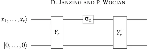
However, our description below will only at one point refer to these results since the observable we construct here is only required to be sparse, in contrast to the k-locality assumed in [25,23]. In some analogy to [16,25] we construct a circuit U that is obtained from Yras follows: First, apply the circuit Yr. Second, apply aσz-gate. Third, implement Yr†. The resulting circuit U is shown in Figure 1. We denote the dimension of the Hilbert space U acts on by ˜N.
|x1, . . . ,xri
Yr
σz
Yr† |0, . . . ,0i
Figure 1:Circuit U constructed from the original circuit Yr. Whenever the answer to the BQP problem is no, the output state of U is close to the input state|x,0i ≡ |x1, . . . ,xn,0, . . . ,0i. Otherwise, the state|x,0iis only restored after applying U twice.
output probabilities of the original circuit. We assume furthermore that M is odd, which is automatically satisfied if we decompose Yr†in analogy to Yrand implement aσz-gate between Yrand Yr†. We define the unitary matrix
W := M−1
∑
`=0
|`+1ih`| ⊗U`, (6.1)
acting onCM⊗CN˜. Here the+sign in the index has always to be read modulo M. We obtain
WM= M−1
∑
`=0
|`ih`| ⊗U`+M· · ·U`+1U`.
Because U2 =1 we have (WM)2 =1. Thus, WM can only have the eigenvalues ±1. This defines a decomposition of the spaceCM⊗CN˜ into symmetric and antisymmetric W -invariant subspacesS+ and S−, respectively with corresponding projectors
Q±:=1 2(1±W
M).
In the following we use the definition|sxi:=|0i ⊗ |x,0ifor the initial state and restrict attention to the
span of the orbit
n
W`|sxio with`∈N. (6.2)
Moreover, we use the abbreviationsα0=αx,0andα1=αx,1. We consider first the two extreme cases |α1|=0 and|α1|=1. If|α1|=0 the orbit (6.2) is M-periodic and the action of W is isomorphic to the action of a cyclic shift in M dimensions, i. e., the mapping|`i 7→ |(`+1)mod Mi, where|`icorresponds to W`|sxiwith`=0,1, . . . ,M−1.
If |α1|=1 the action of W corresponds to a cyclic shift with an additional phase −1, i. e., the mapping|`i 7→ |`+1ifor`=0,1, . . . ,M−2 and|M−1i 7→ −|0i. In the first case, the state|sxiinduces
a spectral measure R(0)being equal to the uniform distribution on the Mth roots of unity, i. e., the values exp(−iπ2`/M)for`=0, . . . ,M−1. In the second case, |sxi induces the measure R(1)being equal to
the uniform distribution on the values exp(−iπ(2`+1)/M)for`=0, . . . ,M−1. We observe that R(1)
and R(0)coincide up to a reflection of the real axis in the complex plane.
In the general case, the orbit defines an 2M-dimensional space whose orthonormal basis vectors are obtained by renormalizing the vectors
We obtain then a convex sum of R(0)and R(1)as spectral measures induced by W and|sxi. The following
calculation shows that|α0|2and|α1|2define the corresponding weights:
hsx|Q+|sxi=
1
2hsx|1+W M|s
xi=
1
2hx,0|1+U|0,xi= 1
2(1+hx,0|Y †
rσzYr|0,x)i=|α0|2,
where the last equality follows easily by replacing Yr|x,0iand its adjoint with the expression in Equa-tion (2.1) and its adjoint. Thus, we obtain the spectral measure
R :=|α0|2R(0)+|α1|2R(1).
We define the self-adjoint operator
A :=1
2(W+W
†). (6.3)
The support of the spectral measure corresponding to A is directly given by the real part of the support of R. To obtain the corresponding probabilities one has to take into account that in many cases two different eigenvalues of W lead to the same eigenvalue of A.
To calculate the distribution of outcomes for A-measurements we observe that R(0)leads to a distri-bution P(0)on the(M−1)/2 eigenvalues
λ`(0)=cos2π`
M for`=0, . . . ,(M−1)/2
with probabilities P1(0):=1/M and P`(0):=2/M for` >1. Likewise, R(1)leads to a distribution P(1)on the(M−1)/2 values
λ`(1)=cosπ(2`+1)
M for`=0, . . . ,(M−1)/2
with probabilities P((M1)−1)/2=1/M and P`(1)=2/M for` <(M−1)/2. As it was true for R(0)and R(1),
the measures P(0)and P(1)coincide up to a reflection.
We now set|ji:=|sxi, i. e., the input state is considered as the jth basis vector ofCM⊗CN˜. Then the diagonal entry(Am)j jcoincides with the mth moment of the spectral measure:
(Am)j j=hj|Am|ji=
∑
λ
λmP(λ),
whereλ runs over all eigenvalues of the restriction of A to the smallest A-invariant subspace containing
|ji, and P(λ) denotes its probability according to the spectral measure corresponding to A. Since the
latter is a convex sum of P(0)and P(1)we may write(Am)j jas the convex sum
(Am)j j = (1− |α1|2)
∑
`
λ`(0)
m
P`(0)+|α1|2
∑
`
λ`(1)
m Pl(1)
=: (1− |α1|2)E0+|α1|2E1. (6.4)
In order to see how the value(Am)j jchanges with|α1|we observe that,
E0= (M−1)/2
∑
`=0
λ`(0)
m
P`(0)≥P0(0)+λ((M0)−1)/2
m
= 1
M+
λ((M0)−1)/2
m .
Here we have used thatλ0(0)=1 and that the eigenvalues are numbered in a decreasing order. Thus, λ(M−1)/2 is the smallest one. Because of the reflection symmetry of the measures we have E1=−E0. Now we choose m sufficiently large such that the term(λ((M0)−1)/2)mis negligible compared to 1/M since
we have then E0−E1≈2/M which is a sufficient difference for our purpose. In order to achieve this we set m :=M3. We have
λ((M0)−1)/2=−cos(π/M)>−1+ π
2
2M2−
π4
4! M4 >−1+
π2
4 M2,
where the last inequality holds for sufficiently large M. Due to
lim M→∞(1−
π2
4 M2)
M2 =e−π2
4
we conclude that
(cos(π/M))M
3
<(e−π
2 4 )M,
and hence
E0> 1 M−(e
−π2
4 )M> 3
4M, (6.5)
where we have, again, assumed M to be sufficiently large. To see how (Am)j j changes with |α1|we recall
(Am)j j= (1− |α1|2)E0+|α1|2E1= (1−2|α1|2)E0,
by Equation (6.4) and the reflection symmetry. Using the worst cases |α1|2=1/3 for x∈ΠNO and |α1|2=2/3 for x∈ΠYESwe obtain
(Am)j j= 1
3E0 and (A
m) j j=−
1 3E0. Using E0>3/(4M)from Equation (6.5) we obtain
(Am)j j> 1 4M,
if the answer is no and
(Am)j j<− 1 4M
otherwise. Setting g :=0 (seeDefinition 4.1) we may defineε :=1/(4 M). Then the diagonal entry is
greater than g+εif x∈ΠYESand smaller than g−εif x∈ΠNO. The construction of A as the real part of a unitary matrix ensures thatkAk ≤1=: b. This shows that we can find an inverse polynomial accuracy
It remains to show that A is row-sparse and column-sparse in the sense defined inSection 4. First we observe the following. For a gate U`that only acts on k qubits non-trivially, the matrix describing U` contains only non-zero entrieshb|U`|b0ifor those pairs b,b0of binary words for which b and b0 differ at most at these k positions. For a given b, one can efficiently check which one of these possible 2kentries is non-zero and similarly for a given b0. Hence we have shown sparseness of U`. It is easy to show that sparseness is also true for W as defined in Equation (6.1) using the gates U`and also for A as defined in Equation (6.3).
Note that estimating of off-diagonal entries only is also PromiseBQP-hard. This can be seen by replacing the original matrix A with
A0:=A⊗
1/2 1/2 1/2 1/2
,
which has obviously the same norm as A since the right-hand matrix is an orthogonal projector. Then we have
(A0)m=Am⊗
1/2 1/2 1/2 1/2
.
We obtain
(Am)j j=2hj,0|(A0)m|j,1i,
where we have used the short-hand notation|j,ii:=|ji ⊗ |iifor i=0,1. Hence we have reproduced the diagonal entry of Amby an off-diagonal entry of(A0)m.
7
Restriction to matrices with entries 0,1,-1
So far we have allowed for general real-valued matrix entries. We may strengthen the result of the preceding section in the sense that diagonal entry estimation remains PromiseBQP-hard if only the entries 0,±1 are possible.
It is known that Toffoli and Hadamard gates are universal for quantum computation [1] (in the sense of encoded universality) . For our purposes, the following modified universal set is useful. Let T and H denote the set of Toffoli gates and the set of Hadamard gates, respectively. We consider Tleft∪Tright∪H, where we have defined Tleft:=T H and Tright:=HT . In words, Tleftis, for instance, the set of gates that are obtained by applying an arbitrary Toffoli-gate followed by a Hadamard gate on an arbitrary qubit. One checks easily that all gates in the universal set Tright∪Tleft∪H have only entries 0,±1/
√ 2. To construct our new version of the matrix A we replace the gates of Yrwith gates taken from our universal set. The problem is that we should simulateσzusing an odd number of gates. Since it is by no means obvious whether and how this could be achieved we replaceσzwith a gate from Tleft∩Tright. The latter is a tensor product of a Hadamard and a Toffoli gate. The Hadamard gate acts on some extra qubit (prepared in the state|0i) that is not used in the computation. The Toffoli gate copies the output to an additional qubit (this is done by initializing a third additional qubit to|1i). One verifies easily that the unitary matrix W defined by these replacements acts as a shift in 2M dimensions whenever the output is 1. We obtain then a uniform mixture of the two spectral measures P(0)and P(1)defined in Section6
of the Hadamard gate define a decomposition of the initial state into two components. On the first component W acts as an M-dimenisonal shift and on the second as a M-dimensional shift with phase factor−1. Therefore we obtain also a mixture of the form r0P(0)+ (1−r0)P(1). But now the weight r0 is equal to 1/(4−2√2) =|h0|ψ+i|2 where|ψ+i is the eigenvector of the Hadamard gate for the
eigenvalue 1. The difference between the diagonal entries of Amfor YES-instances and NO-instances is thus only reduced by a constant factor and the problem remains PromiseBQP-hard.
By rescaling with√2 we obtain a matrix A with entries 0,±1. The rescaling is clearly irrelevant for the diagonal entry estimation problem since we now have spectral values within the interval[−√2,√2] and the accuracy required byDefinition 4.1changes by the factor(√2)maccordingly.
8
Conclusions
We have shown that the estimation of diagonal entries of powers of symmetric sparse matrices is PromiseBQP-complete when the demanded accuracy scales appropriately with the powers of the op-erator norm.
The quantum algorithm proposed here for solving this problem uses the fact that measurements of the corresponding observable allow us to obtain enough information on the probability measure defined by the eigenvector decomposition of the considered basis state. Given the assumption that PromiseBQP6= PromiseBPP, i. e., that a quantum computer is more powerful than a classical computer, the required information on the spectral measure cannot be obtained by any efficient classical algorithm. This is remarkable since the determination of spectral measures is a problem whose relevance is not restricted to applications in quantum theory only.
Acknowledgements
P.W. was supported by the Army Research Office under Grant No. W911NF-05-1-0294 and by the National Science Foundation under Grant No. PHY-456720. This work was begun during D.J.’s visit to the Institute for Quantum Information at the California Institute of Technology. The hospitality of the IQI members is gratefully acknowledged. We would also like to thank Shengyu Zhang and Andrew Childs for helpful discussions.
References
[1] * D. AHARONOV: A simple proof that Toffoli and Hadamard are quantum universal. 2003. [arXiv:quant-ph/0301040]. 7
[2] * D. AHARONOV AND I. ARAD: The BQP-hardness of approximating the Jones polynomial. 2006. [arXiv:quant-ph/0605181]. 1,3
[4] * D. AHARONOV AND A. TA-SHMA: Adiabatic quantum state generation and statistical zero knowledge. In Proc. 35th Annual ACM Symp. on Theory of Computing, pp. 20–29, 2003. [STOC:10.1145/780542.780546]. 4,5.3
[5] *E. BERNSTEIN ANDU. VAZIRANI: Quantum complexity theory. SIAM Journal on Computing, 26(5):1411–1473, 1997. [SICOMP:10.1137/S0097539796300921]. 6
[6] * D. W. BERRY, G. AHOKAS, R. CLEVE, AND B. C. SANDERS: Efficient quantum al-gorithms for simulating sparse Hamiltonians. Comm. Math. Phys., 270(2):359–371, 2007. [Springer:hk7484445j37r228]. 4,5.3
[7] * D. E. BROWNE AND H. BRIEGEL: One-way quantum computation - a tutorial introduction. 2006. [arXiv:quant-ph/0603226]. 1
[8] * A. CHILDS: Quantum information processing in continuous time. PhD thesis, Massachusetts Institute of Technology, 2004. 4,5.3
[9] * A. M. CHILDS, D. W. LEUNG, AND M. A. NIELSEN: Unified derivations of measurement-based schemes for quantum computation. Phys. Rev. A, 71:032318, 2005. [PRA:10.1103/PhysRevA.71.032318]. 1
[10] *S. EVEN, A. L. SELMAN,ANDY. YACOBI: The complexity of promise problems with applica-tions to public-key cryptography. Inform. and Control, pp. 159–173, 1984. 2
[11] *M. FREEDMAN, A. KITAEV,ANDZ. WANG: Simulation of topological field theories by quan-tum computers. Comm. Math. Phys., 227(3):587–603, 2002. [Springer:btldwt3g5t0308da]. 3
[12] *O. GOLDREICH: On promise problems. Technical Report 18, Electr. Colloquium Computational
Complexity, 2005. [ECCC:TR05-018]. 2
[13] * W. HOEFFDING: Probability inequalities for sums of bounded random variables. Journ. Am. Stat. Ass., 58(301):13–30, 1963. 5.2
[14] * D. JANZING: Spin-1/2 particles moving on a 2d lattice with nearest-neighbor interac-tions can realize an autonomous quantum computer. Physical Review, A(75):012307, 2007. [PRA:10.1103/PhysRevA.75.012307]. 1
[15] *D. JANZING ANDP. WOCJAN: Ergodic quantum computing. Quant. Inf. Process., 4(2):129–158, 2005. [Springer:wq1g61v1236574t4]. 1
[16] *D. JANZING, P. WOCJAN, ANDT. BETH: “Non-Identity check” is QMA-complete. Int. Journ. Quant. Inf., 3(3):463–473, 2005. [doi:10.1142/S0219749905001067]. 6
[17] * J. KEMPE, A. KITAEV, AND O. REGEV: The complexity of the local Hamiltonian problem.
SIAM J. Computing, 35(5):1070–1097, 2006. [SICOMP:10.1137/S0097539704445226]. 1,6
[19] *E. KNILL ANDR. LAFLAMME: Quantum computation and quadratically signed weight enumer-ators. Inf. Process. Lett., 79(4), 2001. [IPL:10.1016/S0020-0190(00)00222-2]. 1,3
[20] *M. NIELSEN ANDI. CHUANG: Quantum Computation and Quantum Information. Cambridge University Press, 2000. 5.1,5.1
[21] *R. OLIVEIRA ANDB. TERHAL: The complexity of quantum spin systems on a two-dimensional square lattice. 2005. [arXiv:quant-ph/0504050]. 1,6
[22] * R. RAUSSENDORF AND H. BRIEGEL: A one-way quantum computer. Phys. Rev. Lett.,
86(22):5188–5191, 2001. [PRL:10.1103/PhysRevLett.86.5188]. 1
[23] * P. WOCJAN, D. JANZING, TH. DECKER, ANDTH. BETH: Measuring 4-local n-qubit
observ-ables could probabilistically solve PSPACE. In Proc. Winter International Symp. on Information and Communication Technologies, 2004. (Proceedings contain only the abstract). [arXiv:quant-ph/0308011]. 3,6
[24] * P. WOCJAN AND J. YARD: The Jones polynomial: quantum algorithms and applications in quantum complexity theory. 2006. [arXiv:quant-ph/0603069]. 1,3
[25] * P. WOCJAN AND S. ZHANG: Several natural BQP-complete problems. 2006. [ arXiv:quant-ph/0606179]. 1,3,4,6
AUTHORS
Dominik Janzing[About the author] Fakult¨at f¨ur Informatik
Universit¨at Karlsruhe (TH) Am Fasanengarten 5 76 131 Karlsruhe Germany
janzing ira ura de
http://iaks-www.ira.uka.de/home/janzing/
Pawel Wocjan[About the author]
School of Electrical Engineering and Computer Science University of Central Florida
Orlando
FL 32816, USA wocjan cs ucf edu
ABOUT THE AUTHORS
DOMINIK JANZING studied physics and mathematics in T¨ubingen (Germany) and Cork (Ireland). His main interests were the foundations of quantum theory and thermody-namics. In 1998, he completed his Ph. D. thesis under the supervision of Manfred Wolff on the relation between quantum and classical dynamics in infinite quantum spin chains. When he joined the quantum computing group of Thomas Beth in the Faculty of Com-puter Science at theUniversit¨at Karlsruhehe did not expect that he would ever write a paper on complexity classes since his goal was “only” to understand the limits of quan-tum control. But while he was biking in the forests around Karlsruhe he realized that Pawel’s and his results on the complexity of certain quantum measurements allow us to define a PromiseBQP-complete problem. When he was visiting Pawel at Caltech, the California sun gave both of them the strength to improve this idea. Dominik enjoys hiking, especially when his girlfriend Steffi joins him. He also likes fancy furniture.