Performance Evaluation of Distance Metrics in the Clustering
Algorithms
VIJAYKUMAR1
JITENDERKUMARCHHABRA2
DINESHKUMAR3
1Computer Science & Engineering Department, Manipal University, Jaipur, Rajesthan, INDIA
2Computer Engineering Department, National Institute of Technology, Kurukshetra, Haryana, INDIA
3CSE Department, Guru Jambheshwer University of Science & Technology, Hisar, Haryana, INDIA
1
Abstract. Distance measures play an important role in cluster analysis. There is no single distance measure that best fits for all types of the clustering problems. So, it is important to find set of distance measures for different clustering techniques on datasets that yields optimal results. In this paper, an attempt has been made to evaluate ten different distance measures on eight clustering techniques. The quality of the distance measures has been computed on basis of three factors: accuracy, inter-cluster and intra-cluster distances. The performance of clustering algorithms on different distance measures has been evaluated on three artificial and six real life datasets. The experimental results reveal that the performance and quality of different distance measures vary with the nature of data as well as clustering techniques. Hence choice of distance measure must be done on basis of dataset and clustering technique.
Keywords: Distance Measures; Clustering Algorithms; Ant Colony based Clustering; Modified Har-mony Search Clustering.
(Received May 26th, 2014 / Accepted August 8th, 2014)
1 Introduction
Clustering is an important data mining technique where information about labeling and structure is not avail-able. It is the process of partitioning a set of data points into different groups such that the data in each group are similar to each other. Clustering algorithms are broadly classified into two groups: hierarchical and partitional [7]. Hierarchical clustering algorithms recursively find nested clusters either in agglomerative mode or in divi-sive mode. The former one starts with each data point in its own cluster and merges the most similar pair of clusters successively to form a cluster hierarchy and the latter starts with all the data points in one cluster and recursively divides each cluster into smaller clus-ters [21]. The well-known agglomerative hierarchical
clustering algorithms are single, average, complete and weighted linkage. On the other hand, partitional clus-tering groups the data points into some pre-specified number of clusters without using hierarchical structure. The most popular partitional clustering techniques are K-Means, K-Medoid, Fuzzy C-Means and Expectation-Maximization.
Kumar, Chhabra and Kumar Performance Evaluation of Distance Metrics in the Clustering Algorithms 39
according to another distance [19, 20]. The motivation of this paper is to analyze the effect and evaluate the performance of various distance measures on different clustering techniques.
In this paper, we study the distance measures from a new perspective: how they affect the clustering re-sults. The ten well-known distance measures are dis-cussed with their relative strengths and weaknesses. These are: Euclidean, Standardized Euclidean, Manhat-tan, Mahalanbois, Cosine Similarity, Pearson Correla-tion, Spearman CorrelaCorrela-tion, Chebychev, Canberra, and Bray-Curtis. These are evaluated in conjunction with eight different clustering techniques over nine different datasets. The rest of the paper is organized as follows. Section 2 presents clustering techniques. Section 3 in-troduces distance measures that used for numerical data sets in clustering. In Section 4, the effect of distance measures on clustering techniques is investigated. Fi-nally, a concluding remark is drawn in Section 5.
2 Clustering Techniques
The clustering algorithms are used to partition the dataset X = x1, x2, . . . , xj, . . . , xN, where xj =
(xj1, xj2, . . . , xjd) ∈ Rd into a number of clusters,
sayK,(C1, C2, . . . , CK). The parition matrixU(X)
is represented as U = [ukj], k = 1,2, . . . , K, and j = 1,2. . . , N, where ukj is membership of
dat-apoint xj to clusters Ck. The ukj = 1 if xj ∈ Ck;otherwise, ukj= 0.
2.1 Hierarchical Clustering Techniques
The agglomerative hierarchical clustering techniques have been used in this paper. The well- known ag-glomerative hierarchical techniques are single linkage, average linkage, complete linkage and weighted link-age.
The single linkage clustering is based on the local connectivity criterion [7]. It is also known as a nearest neighbor method. It starts by considering each data point in a cluster of its own. It computes the distances between two clusterspandqsuch as [13]
DSL(p, q) = min xi∈p,xj∈q
{d(xi, xj)} (1)
Based on these distances, it merges the two closest clus-ters and replacing them by one merged cluster. The dis-tances of the remaining clusters from the merged clus-ter are recomputed as mentioned above. This process continues until all the data points are in a single clus-ter. The main advantage of single linkage is that it can handle non-elliptical shapes. However, it is sensitive to-wards noise and outliers [7, 18].
The average linkage clustering has a similar procedure as the single linkage except the distance computation between two clusters. It uses the average of pairwise distance between points in two clusterspandqas:
DAL(p, q) =
1
|p||q| X
xi∈p
X
xj∈q
d(xi, xj) (2)
It is less susceptible to noise and outliers. The one dis-advantage is its biasing towards globular clusters [18]. The complete linkage clustering is also called the fur-thest method. It uses the largest distance between data points in two clusterspandqas:
DCL(p, q) = max xi∈p,xj∈q
{d(xi, xj)} (3)
It does not account for cluster structure. It cannot de-tect the non-spherical clusters. The weighted average linkage method is also known as weighted pair group method using arithmetic average. The difference be-tween average and weighted linkage is that the dis-tances between the newly formed cluster and the rest are weighted based on the number of data points in each cluster.
2.2 Partitional Clustering Techniques
The well-known partitional techniques are K-Means and K-Mediods. The main disadvantages of these tech-niques are that these are easily trapped in local optima. The K-Means is well-known partitional clustering al-gorithm [7]. It seeks an optimal partition of data by minimizing the sum-of-squared-error criterion with an iterative optimization procedure such as [7, 13]
J(U, V) =
N X
j=1
K X
i=1
uijkxj−vik2 (4)
whereviis the center of clusterCi. Here, cluster
cen-ters are initialized by randomly chosen data points form dataset. Each data point is assigned to the nearest clus-ter using minimum distance criclus-terion. Thereafclus-ter, the cluster centers are updated to the mean of data points belonging to them. This process is repeated until there is no change for each cluster. The disadvantage of K-Means is that it is sensitive towards initialization of cluster centers.
The K-Medoid algorithm is an adaptation of K-Means algorithm. Rather than calculating the mean of data points in each cluster, medoid is chosen for each cluster at each iteration.
Shelokar et al. [17] described an ant colony optimiza-tion methodology for data clustering (ACOC). It mainly
relies on pheromone trails to guide ants to group data points according to their similarity and on a local search that randomly tries to improves the best iteration solu-tion before updating pheromone trails.
Kumar et al. [9, 10] developed a modified harmony search based clustering (M HSC) technique. Here cluster center based encoding scheme is used. Each harmony vector containsK cluster centers, which are initialized toKrandomly chosen data points from the given dataset. This process is repeated for each of the HM S vectors in the harmony memory, where HM S is the harmony memory size. The data points are as-signed to different cluster centers based on minimum Euclidean distance criterion and cluster centers repre-sented by the harmony vectors are replaced by the mean data points of respective clusters. The fitness of each harmony vectors is computed using sum-of-squared-error criterion and is minimized using modified har-mony search algorithm. The improvisation process is used to update the harmony vectors. In M HSC, the processes of fitness computation and improvisation are executed for a maximum number of iterations. The best harmony vector at the end of last iteration provides the solution to the clustering problem.
3 Distance Measures
The distance measure must be determined before the clustering. It reflects the degree of separation among target data points and should correspond to the charac-teristics used to distinguish the clusters embedded in the dataset [6, 3]. These characteristics are data dependent in most of cases. There is no single distance measure that is best for all types of clustering problems. There-fore, understanding the importance of different distance measures will help us to choose the best one. Every dis-tance measure is not a metric. To qualify as a metric, a measure must satisfy the following four conditions [7, 21].
1. The distance between any two data points must be non-negative, i.e.,
D(xi, xj)≥0for allxiandxj
2. The distance between two data points must be zero if and only if the two data points are identical, i.e., D(xi, xj) = 0if and only ifxi=xj
3. The distance fromxitoxj is the same as the
dis-tance fromxjtoxi, i.e., D(xi, xj) =D(xj, xi)
4. The distance measure must satisfy the triangle in-equality, which is
D(xi, xj) +D(xj, xk)≥D(xi, xk)for allxi,xj
andxk.
3.1 Euclidean Distance
The Euclidean distance is most commonly used dis-tance measure. It is also known asL2norm. The Eu-clidean distance,De, between two data pointsxi and xjis defined as:
De(xi, xj) = d X
l=1
|xil−xjl|2 !12
(5)
wherexilandxjlrepresent thelthdimension ofxiand xj respectively. It tends to form hyperspherical
clus-ters. It satisfies all the above mentioned four conditions and therefore is a metric [21]. The strength of this mea-sure is that clusters formed are invariant to translation and rotation in the feature space. This measure has dis-advantages also. If one of the input attributes has a rel-atively large range, then it can overcome the other at-tributes [21].
3.2 Standardized Euclidean Distance
The standardized Euclidean distance is defined as the Euclidean distance between the data points divided by their standard deviation. The squared standardized Eu-clidean distance betweenxi andxj is mathematically
described as:
DSe(xi, xj) = (xi−xj)D−1(xi−xj)T (6)
whereDis the diagonal matrix with diagonal elements are given byva2j, which represents the variance of vari-ablexj over N data points. This measure is a metric
as it satisfies the conditions of metric. When squared standardized Euclidean distance is multiplied by the ge-ometric mean of the variances, it produces a diagonal Mahalanobis distance measure. The diagonal Maha-lanobis distance fails to use the information of the di-agonal in the covariance matrix [16].
3.3 Manhattan Distance
Manhattan distance between two data points is defined as the sum of the absolute differences of their coordi-nates. It is also known as a city block, rectilinear, taxi-cab orL1distance. It is mathematically defined as:
DM n(xi, xj) = d X
l=1
|xil−xjl| (7)
Kumar, Chhabra and Kumar Performance Evaluation of Distance Metrics in the Clustering Algorithms 41
of dataset are binary in nature, the Manhattan distance acts as a Hamming distance [7]. It is also a metric. The advantage of over Euclidean distance is the reduced computation time [7]. Further it does not depend upon the translation and reflection of the coordinate system. The one disadvantage is that it depends upon the rota-tion of the coordinate system.
3.4 Mahalanbois Distance
Mahalanobis [12] introduced a new distance measure named as Mahalanobis distance. It is also known as quadratic distance. It is based on the correlations be-tween variables by which different patterns can be iden-tified and analyzed. The Mahalanobis distance is de-fined as:
DM a(xi, xj) = (xi−xj)V−1(xi−xj)T (8)
whereV is covariance matrix. If the covariance matrix is identity matrix, the Mahalanobis distance reduces to the Euclidean distance. It differs from the Euclidean distance in that it takes into account the correlations of the dataset and is scale-invariant. It leads to vio-lations of the triangle inequality and sensitive towards sampling fluctuations (Cherry et al., 1982). The Maha-lanobis distance tends to form ellipsoidal clusters.
3.5 Cosine Distance
Cosine distance is a measure of dissimilarity between two vectors by measuring the cosine of the angle be-tween them. It is defined as
Dcos(xi, xj) = 1− xT
ixj kxikkxjk
(9)
It is bounded between 0 and 1 if and are non-negative. It is used to measure cohesion within clusters [18]. This measure is not a distance metric and violates the trian-gle inequality. It is also invariant to scaling. It is unable to provide information on the magnitude of the differ-ences. It is not invariant to shifts.
3.6 Correlation Distance
The correlation distance measure is derived from the Pearson correlation coefficient [8]. The correlation co-efficient is used to measure the degree of linear depen-dency between two data points. The correlation based distance measure is mathematically formulated as:
DCorr(xi, xj) = 1−SCR(xi, xj) (10)
SCR(xi, xj) =
Pd
k=1(mik)(mjk) q
Pd
k=1(mik)2
Pd
k=1(mjk)2 (11)
where mik = xik −xi, mjk = xjk −xj, xi =
1
d Pd
k=1xik andxj = 1d Pd
k=1xjk. This measure is
not a distance metric. It tends to disclose the difference in shapes rather than to detect the magnitude of differ-ences between two data points [21]. It is invariant to both scaling and translation.
3.7 Spearman Distance
The Spearman distance measure is derived from the Spearman correlation coefficient [5]. It can be defined as
DSpear(xi, xj) = 1−SC(xi, xj) (12)
SC(xi, xj) =
Pd k=1(m
r ik)(m
r jk) q
Pd k=1(m
r ik)2
Pd k=1(m
r jk)2
(13)
wheremr
ik = r(xik)−r, mrjk = r(xjk)−r. In
Spearman rank correlation, each data value is replaced by their rank if the data in each vector is ordered by its value. Then Pearson correlation between the two rank vectors is computed instead of the data vectors. The Spearman rank correlation is an example of a non-parametric similarity measure. It is robust against out-liers than the Pearson correlation. The disadvantage is that there is a loss of information when data are con-verted to ranks.
3.8 Chebyshev Distance
The Chebyshev distance calculates the maximum of the absolute differences between the features of a pair of data points. This distance is named after Panfnuty Chebyshev. It is also known as tchebyschev distance, maximum metric, chessboard distance, or metric. It is mathematically defined as
DCh(xi, xj) =max1≤l≤d(|xil−xjl|) (14)
This distance measure is a metric. The advantage is that it takes less time to decide the distances between data sets [15].
3.9 Canberra Distance
Lance and Williams [11] introduced a Canberra dis-tance measure. It measures the sum of absolute frac-tional differences between the features of a pair of data points. It is mathematically defined as follows:
DCan(xi, xj) = d X
l=1
|xil−xjl|
|xil|+|xjl| (15)
This distance measure is a metric. It is sensitive to a small change when both coordinates are near to zero.
3.10 Bray-Curtis Distance
The Bray-Curtis distance is also known as Sorensen dis-tance [2]. This measure is computed using the absolute differences divided by the summation. It is defined as follows:
DBc(xi, xj) = Pd
l=1|xil−xjl| Pd
l=1(xil+xjl)
(16)
This distance measure is not a metric as it does not sat-isfy the triangle inequality property. The main draw-back of this measure is that it is undefined if both data points are near zero values.
4 Experimental Results
This section provides a description of the datasets and demonstrate the efficiency of well-known clustering algorithms based on ten different distance measures. The results are evaluated and compared using some widely acceptable performance evaluation metrics such as accuracy, inter-cluster and intra-cluster distance [4]. Large value of accuracy measure is required for bet-ter clusbet-tering. Smaller value of intra-clusbet-ter and large value of inter-cluster distance is required for better clus-tering. All the results are evaluated in terms of ’mean’ and ’standard deviation’. The standard deviation is used as a measure of robustness, which is shown in parenthe-sis.
4.1 Datasets used
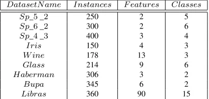
Experiments are carried out with three artificial and six real-life datasets. A description of datasets is depicted in Table 1. The artificial datasets are named as Sp_4 _3,Sp_5 _2 andSp_6_2. These are taken from [1]. The six real-life datasets are obtained from UCI ma-chine learning database [14].
Table 1:Description of Datasets Used
DatasetN ame Instances F eatures Classes
Sp_5_2 250 2 5
Sp_6_2 300 2 6
Sp_4_3 400 3 4
Iris 150 4 3
W ine 178 13 3
Glass 214 9 6
Haberman 306 3 2
Bupa 345 6 2
Libras 360 90 15
4.2 Parameter setting for the algorithms
The K-Means and K-Medoid were executed for 100 it-erations. The parameters of the ACOC are as follows: evaporation rate = 0.1, number of ants = 20, and maxi-mum number of iterations = 100 as mentioned in [17]. The parameters of the MHSC are as follows: harmony memory size = 15 and maximum number of iterations = 100. The pitch adjustment rate, harmony memory con-sideration rate and bandwidth are chosen as in [9, 10]. The value ofK, number of clusters, for datasets equals the number of classes of the corresponding datasets as mentioned in Table 1.
4.3 Experimentation 1: Effect of distance mea-sures on Hierarchical Techniques
Tables 2-10 show the effect of distance measures on ac-curacy forSp_5 _2, Sp_6_2,Sp_4 _3,Iris, W ine, Glass,Haberman,BupaandLibrasdatasets respec-tively. The results reported in tables are the average values obtained over ten runs of algorithms. Figures 1-2 show the effect of distance measures on inter and intra-cluster distance.
Figure 1: Effect of distance measures on Inter-cluster distance for hierarchical techniques; (a)Sp_5_2(b)Sp_6_2(c)Sp_4_3(d) Iris(e)W ine(f)Glass(g)Glass(h)Haberman(i)Bupa.
Figure 2: Effect of distance measures on Intra-cluster distance for hierarchical techniques; (a)Sp_5_2(b)Sp_6_2(c)Sp_4_3(d) Iris(e)W ine(f)Glass(g)Glass(h)Haberman(i)Bupa.
Kumar, Chhabra and Kumar Performance Evaluation of Distance Metrics in the Clustering Algorithms 43
Table 2:Effect of distance measures on accuracy of cluster formed forSph_5_2dataset for Hierachical Clustering Techniques
Dist.M eas. S.Lin. C.Lin. A.Lin. W.Lin. Eucl. 0.596 0.948 0.940 0.956
(0.000) (0.000) (0.000) (0.000)
S.Eucl. 0.588 0.848 0.948 0.948
(0.000) (0.000) (0.000) (0.000)
M anh. 0.356 0.940 0.944 0.860
(0.000) (0.000) (0.000) (0.000)
M ahal. 0.588 0.928 0.948 0.912
(0.000) (0.000) (0.000) (0.000)
Cos. 0.464 0.488 0.508 0.556
(0.000) (0.000) (0.000) (0.000)
Corr. 0.400 0.416 0.404 0.408
(0.000) (0.000) (0.000) (0.000)
Spear. 0.400 0.400 0.400 0.400
(0.000) (0.000) (0.000) (0.000)
Cheb. 0.420 0.892 0.932 0.896
(0.000) (0.000) (0.000) (0.000)
Canb. 0.216 0.736 0.944 0.812
(0.000) (0.000) (0.000) (0.000)
Bray 0.204 0.964 0.964 0.720
(0.000) (0.000) (0.000) (0.000)
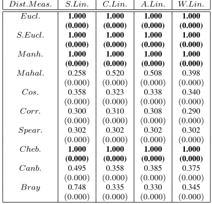
Table 3:Effect of distance measures on accuracy of cluster formed forSph_6_2dataset for Hierarchical Clustering Techniques
Dist.M eas. S.Lin. C.Lin. A.Lin. W.Lin. Eucl. 1.000 1.000 1.000 1.000
(0.000) (0.000) (0.000) (0.000)
S.Eucl. 1.000 1.000 1.000 1.000 (0.000) (0.000) (0.000) (0.000)
M anh. 1.000 1.000 1.000 1.000 (0.000) (0.000) (0.000) (0.000)
M ahal. 1.000 1.000 1.000 1.000 (0.000) (0.000) (0.000) (0.000)
Cos. 0.483 0.560 0.577 0.577
(0.000) (0.000) (0.000) (0.000)
Corr. 0.320 0.340 0.340 0.323
(0.000) (0.000) (0.000) (0.000)
Spear. 0.320 0.320 0.320 0.320
(0.000) (0.000) (0.000) (0.000)
Cheb. 1.000 1.000 1.000 1.000 (0.000) (0.000) (0.000) (0.000)
Canb. 0.827 0.760 0.810 0.760
(0.000) (0.000) (0.000) (0.000)
Bray 0.813 0.760 0.760 0.760
(0.000) (0.000) (0.000) (0.000)
For Sph_6 _2 dataset (Table 3), all above-mentioned hierarchical clustering techniques provide well-separated and compact clusters with 100 percent accuracy using five distance measures as Euclidean, Standard Euclidean, Manhattan, Mahalanobis, and Chebychev.
From Table 4, Figures 1(c) and 2(c), it is observed
Table 4:Effect of distance measures on accuracy of cluster formed forSph_4_3dataset for Hierarchical Clustering Techniques
Dist.M eas. S.Lin. C.Lin. A.Lin. W.Lin. Eucl. 1.000 1.000 1.000 1.000
(0.000) (0.000) (0.000) (0.000)
S.Eucl. 1.000 1.000 1.000 1.000 (0.000) (0.000) (0.000) (0.000)
M anh. 1.000 1.000 1.000 1.000 (0.000) (0.000) (0.000) (0.000)
M ahal. 0.258 0.520 0.508 0.398
(0.000) (0.000) (0.000) (0.000)
Cos. 0.358 0.323 0.338 0.340
(0.000) (0.000) (0.000) (0.000)
Corr. 0.300 0.310 0.308 0.290
(0.000) (0.000) (0.000) (0.000)
Spear. 0.302 0.302 0.302 0.302
(0.000) (0.000) (0.000) (0.000)
Cheb. 1.000 1.000 1.000 1.000 (0.000) (0.000) (0.000) (0.000)
Canb. 0.495 0.358 0.385 0.375
(0.000) (0.000) (0.000) (0.000)
Bray 0.748 0.335 0.330 0.345
(0.000) (0.000) (0.000) (0.000)
that all above-mentioned hierarchical clustering tech-niques provide well-separated and compact clusters with 100 percent accuracy using four distance mea-sures (Euclidean, Standard Euclidean, Manhattan, and Chebychev) forSph_4_3dataset.
Table 5:Effect of distance measures on accuracy of cluster formed forIrisdataset for Hierarchical Clustering Techniques
Dist.M eas. S.Lin. C.Lin. A.Lin. W.Lin. Eucl. 0.680 0.840 0.907 0.900
(0.000) (0.000) (0.000) (0.000)
S.Eucl. 0.660 0.787 0.687 0.567
(0.000) (0.000) (0.000) (0.000)
M anh. 0.673 0.893 0.900 0.953
(0.000) (0.000) (0.000) (0.000)
M ahal. 0.353 0.413 0.347 0.607
(0.000) (0.000) (0.000) (0.000)
Cos. 0.660 0.840 0.660 0.960
(0.000) (0.000) (0.000) (0.000)
Corr. 0.660 0.853 0.947 0.687
(0.000) (0.000) (0.000) (0.000)
Spear. 0.673 0.673 0.673 0.673
(0.000) (0.000) (0.000) (0.000)
Cheb. 0.680 0.813 0.733 0.740
(0.000) (0.000) (0.000) (0.000)
Canb. 0.627 0.960 0.627 0.687
(0.000) (0.000) (0.000) (0.000)
Bray 0.660 0.893 0.693 0.827
(0.000) (0.000) (0.000) (0.000)
ForIris dataset (Table 5), the single linkage with Euclidean or Chebyshev distance attains better
racy than the other distance measures. However, it produces well-separated clusters with Mahalanobis dis-tance (Figure 1(d)). From Figure 2(d), it has been found that single linkage gives compact clusters with four dis-tance measures (Standard Euclidean, Cosine, Correla-tion, and Bray-Curtis). The complete linkage with Can-berra distance provides higher accuracy than the other distances. It offers best cluster separation and compact-ness with Spearman distance (Figures 1(d) and 2(d)). The average linkage clustering with Correlation dis-tance attains best accuracy. However, it gives well-separated clusters with Mahalanobis and compact clus-ters with Cosine distance. The weighted linkage using Cosine distance offeres best accuracy among other dis-tance measures. It provides compact and best cluster separation with Spearman distance.
Table 6:Effect of distance measures on accuracy of cluster formed forW inedataset for Hierarchical Clustering Techniques
D.M eas. S.Lin. C.Lin. A.Lin. W.Lin. Eucl. 0.427 0.674 0.612 0.562
(0.000) (0.000) (0.000) (0.000)
S.Eucl. 0.376 0.837 0.388 0.618
(0.000) (0.000) (0.000) (0.000)
M anh. 0.399 0.674 0.545 0.635
(0.000) (0.000) (0.000) (0.000)
M ahal. 0.388 0.371 0.388 0.371
(0.000) (0.000) (0.000) (0.000)
Cos. 0.410 0.562 0.448 0.483
(0.000) (0.000) (0.000) (0.000)
Corr. 0.388 0.685 0.472 0.545
(0.000) (0.000) (0.000) (0.000)
Spear. 0.387 0.612 0.612 0.589
(0.000) (0.000) (0.000) (0.000)
Cheb. 0.427 0.657 0.612 0.545
(0.000) (0.000) (0.000) (0.000)
Canb. 0.387 0.652 0.646 0.646
(0.000) (0.000) (0.000) (0.000)
Bray 0.399 0.719 0.725 0.573
(0.000) (0.000) (0.000) (0.000)
For W ine dataset, the single linkage with Eu-clidean or Chebychev distance produces well-separated clusters having optimal accuracy. It gives compact clusters with Bray-Curtis or City-Block distance (Figure 2(e)). The complete linkage with Standard Euclidean distance attains higher accuracy as compared to other distance measures. It produces well-separated clusters with Correlation distance (Figure 1(e)). The single and complete linkage produce compact clusters with Bray-Curtis distance. The average linkage with Bray-Curtis attains higher accuracy. The average linkage provides well-separated cluster with Euclidean or Chebychev distance and compact clusters with Mahalanobis distance. The weighted linkage with
Canberra distance provides better accuracy than the other distance measures. It produces compact and well-separated clusters with City-Block distance.
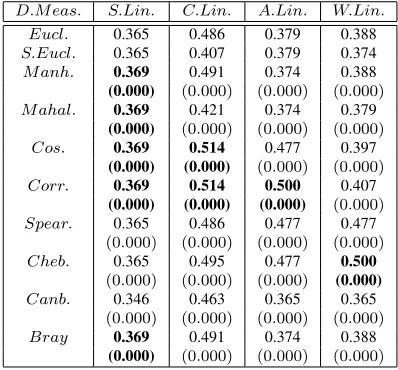
Table 7:Effect of distance measures on accuracy of cluster formed forGlassdataset for Hierarchical Clustering Techniques
D.M eas. S.Lin. C.Lin. A.Lin. W.Lin. Eucl. 0.365 0.486 0.379 0.388 S.Eucl. 0.365 0.407 0.379 0.374 M anh. 0.369 0.491 0.374 0.388
(0.000) (0.000) (0.000) (0.000)
M ahal. 0.369 0.421 0.374 0.379
(0.000) (0.000) (0.000) (0.000)
Cos. 0.369 0.514 0.477 0.397
(0.000) (0.000) (0.000) (0.000)
Corr. 0.369 0.514 0.500 0.407
(0.000) (0.000) (0.000) (0.000)
Spear. 0.365 0.486 0.477 0.477
(0.000) (0.000) (0.000) (0.000)
Cheb. 0.365 0.495 0.477 0.500
(0.000) (0.000) (0.000) (0.000)
Canb. 0.346 0.463 0.365 0.365
(0.000) (0.000) (0.000) (0.000)
Bray 0.369 0.491 0.374 0.388
(0.000) (0.000) (0.000) (0.000)
For Glass dataset, the single linkage clustering provides higher accuracy over five distances (Man-hattan, Mahalanobis, Cosine, Correlation and Bray-Curtis). The complete linkage attains good accuracy with Cosine and Correlation distances. The average linkage with Correlation distance produces superior ac-curacy. The weighted linkage provides better accu-racy using Chebyshev distance. The single, complete, and weighted linkage with Standard Euclidean distance gives well-separated clusters (Figure 1(f)). The av-erage linkage provides well-separated clusters using City-Block or Bray-Curtis distance. The single link-age with Canberra distance generates compact clusters. The complete and weighted linkage with Standard Eu-clidean distance gives clusters with good compactness (Figure 2(f)). The average linkage gives better compact clusters with Mahalanobis distance.
Kumar, Chhabra and Kumar Performance Evaluation of Distance Metrics in the Clustering Algorithms 45
Table 8:Effect of distance measures on accuracy of cluster formed forHabermandataset for Hierarchical Clustering Techniques
D.M eas. S.Lin. C.Lin. A.Lin. W.Lin. Eucl. 0.739 0.556 0.739 0.739
(0.000) (0.000) (0.000) (0.000)
S.Eucl. 0.739 0.748 0.735 0.735
(0.000) (0.000) (0.000) (0.000)
M anh. 0.739 0.742 0.735 0.627
(0.000) (0.000) (0.000) (0.000)
M ahal. 0.739 0.745 0.735 0.739 (0.000) (0.000) (0.000) (0.000)
Cos. 0.739 0.732 0.732 0.732
(0.000) (0.000) (0.000) (0.000)
Corr. 0.739 0.739 0.739 0.739 (0.000) (0.000) (0.000) (0.000)
Spear. 0.739 0.739 0.739 0.739 (0.000) (0.000) (0.000) (0.000)
Cheb. 0.739 0.552 0.735 0.637
(0.000) (0.000) (0.000) (0.000)
Canb. 0.739 0.569 0.582 0.582
(0.000) (0.000) (0.000) (0.000)
Bray 0.739 0.732 0.735 0.739 (0.000) (0.000) (0.000) (0.000)
provides similar accuracy. It produces compact clusters with Canberra distance and well-separated clusters with two distances (Spearman and Correlation).
Table 9:Effect of distance measures on accuracy of cluster formed forBupadataset for Hierarchical Clustering Techniques
D.M eas. S.Lin. C.Lin. A.Lin. W.Lin. Eucl. 0.577 0.577 0.557 0.577
(0.000) (0.000) (0.000) (0.000)
S.Eucl. 0.577 0.559 0.571 0.577 (0.000) (0.000) (0.000) (0.000)
M anh. 0.571 0.574 0.562 0.557
(0.000) (0.000) (0.000) (0.000)
M ahal. 0.577 0.545 0.577 0.577 (0.000) (0.000) (0.000) (0.000)
Cos. 0.577 0.551 0.562 0.565
(0.000) (0.000) (0.000) (0.000)
Corr. 0.577 0.551 0.574 0.551
(0.000) (0.000) (0.000) (0.000)
Spear. 0.577 0.507 0.571 0.571
(0.000) (0.000) (0.000) (0.000)
Cheb. 0.577 0.554 0.557 0.571
(0.000) (0.000) (0.000) (0.000)
Canb. 0.577 0.522 0.562 0.554
(0.000) (0.000) (0.000) (0.000)
Bray 0.577 0.559 0.565 0.554
(0.000) (0.000) (0.000) (0.000)
The results obtained for theBupadataset (Table 9) show that the single linkage clustering produces sim-ilar accuracy for nine distance measures except Man-hattan. It produces well-separated clusters using Maha-lanobis distance and compact clusters using three
dis-tances named as Euclidean, Bray-Curtis, and Cheby-shev (Figures 1(h) and 2(h)). The complete linkage using Euclidean distance produces accurate and com-pact clusters. It provides well-separated clusters with Bray-Curtis. The average linkage using Mahalanobis distance produces accurate and compact clusters. It provides well-separated clusters with City-Block. The weighted linkage attains best accuracy value on Eu-clidean, Standard EuEu-clidean, and Mahalanobis dis-tances. It generates compact clusters with Mahalanobis distance and well-separated clusters with Cosine dis-tance.
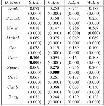
Table 10:Effect of distance measures on accuracy of cluster formed forLibrasdataset for Hierarchical Clustering Techniques
D.M eas. S.Lin. C.Lin. A.Lin. W.Lin. Eucl. 0.072 0.253 0.244 0.183
(0.000) (0.000) (0.000) (0.000)
S.Eucl. 0.075 0.158 0.078 0.256
(0.000) (0.000) (0.000) (0.000)
M anh. 0.078 0.147 0.286 0.267
(0.000) (0.000) (0.000) (0.000)
M ahal. 0.069 0.075 0.069 0.069
(0.000) (0.000) (0.000) (0.000)
Cos. 0.078 0.119 0.189 0.100
(0.000) (0.000) (0.000) (0.000)
Corr. 0.106 0.094 0.164 0.108
(0.000) (0.000) (0.000) (0.000)
Spear. 0.069 0.275 0.256 0.266
(0.000) (0.000) (0.000) (0.000)
Cheb. 0.067 0.261 0.158 0.197
(0.000) (0.000) (0.000) (0.000)
Canb. 0.072 0.068 0.068 0.150
(0.000) (0.000) (0.000) (0.000)
Bray 0.072 0.244 0.139 0.128
(0.000) (0.000) (0.000) (0.000)
ForLibrasdataset results given in Table 10, show that the single linkage clustering using correlation distance provide good accuracy. The single linkage gives well-separated clusters using Cosine. The Complete linkage attains high accuracy over Spearman distance. The average and weighted linkage cluster-ing with Manhattan distance gives better accuracy than the other distances. The complete and average linkage techniques produce well-separated clusters with Bray-Curtis distance (Figure 1(i)). The weighted linkage technique with Chebyshev distance generates separated clusters. Form Figure 2(i), it has been found that Mahalanobis distance provides compact clusters for all hierarchical techniques.
The aforementioned results indicate that the differ-ent distance measures with clustering techniques show different cluster quality value. The summa-rized results for hierarchical clustering techniques in
terms of accuracy, Inter −clusterDistance, and Intra−clusterDistanceare tabulated in Tables 11, 12 and 13.
Table 11:Best distance measures corresponding to datasets and hier-archical clustering techniques in terms of Accuracy
Dataset S.Lin. C.Lin. A.Lin. W.Lin. Sp_5_2 Eucl. Bray Bray Eucl. Sp_6_2 S5 S5 S5 S5
Sp_4_3 Eucl. Eucl. Eucl. Eucl. S.Eucl. S.Eucl. S.Eucl. S.Eucl. M ahal. M ahal. M ahal. M ahal. Cheb. Cheb. Cheb. Cheb. Iris Eucl. Canb. Corr. Cos.
Cheb.
W ine Eucl. S.Eucl. Bray Canb. Cheb.
Glass M ahal. Cos. Corr. Cheb. M anh. Corr.
Corr. Bray Cos.
Haber. All S.Eucl. Corr. Spear Spear Bray Eucl. M ahal.
Eucl. Corr. Bupa All Eucl. M ahal. Eucl.
except S.Eucl.
M anh. M ahal.
Libras Corr. Spear M anh. M anh. CM C Corr. Canb. Cheb. Corr.
Table 12:Best distance measures corresponding to datasets and hier-archical clustering techniques in terms of Inter-cluster Distance
Dataset S.Lin. C.Lin. A.Lin. W.Lin. Sp_5_2 Cheb Corr. Spear Corr. Sp_6_2 S5 S5 S5 S5
Sp_4_3 M ahal. Eucl. Eucl. Eucl. S.Eucl. S.Eucl. S.Eucl. M ahal. M ahal. M ahal. Cheb. Cheb. Cheb. Iris M ahal. Spear M ahal. Spear
Cheb.
W ine Eucl. Canb. Eucl. M anh.
Cheb. Cheb.
Glass S.Eucl. S.Eucl. M anh. S.Eucl. Bray
Haber All Corr. Corr. Corr. Spear Spear Spear Bupa M ahal. Bray M anh. Cos. Libras Cos. Bray Bray Cheb.
Table 13:Best distance measures corresponding to datasets and hier-archical clustering techniques in terms of Intra-cluster Distance
Dataset S.Lin. C.Lin. A.Lin. W.Lin. Sp_5_2 Bray Spear Spear Spear Sp_6_2 S5 S5 S5 S5
Sp_4_3 Eucl. Eucl. Eucl. Eucl. S.Eucl. S.Eucl. S.Eucl. S.Eucl. M ahal. M ahal. M ahal. M ahal. Cheb. Cheb. Cheb. Cheb. Iris S.Eucl. Spear Cos. Spear
Cos. Corr.
W ine M anh. Bray M ahal. M anh. Bray
Glass Canb. S.Eucl. M ahal. S.Eucl. Haber. All Corr. Corr. Canb.
Spear Spear
Bupa Eucl. Eucl. M ahal. M ahal. Bray
Cheb.
Libras M ahal. M ahal. M ahal. M ahal.
4.4 Experimentation 2: Effect of distance mea-sures on Partitional Techniques
Tables 14-22 show the effect of distance measures on accuracy forSp_5_2,Sp_6_2,Sp_4_3,Iris,W ine, Glass,Haberman,BupaandLibrasdatasets respec-tively. The results reported in tables are the average values obtained over ten runs of algorithms. Figures 3-4 show the effect of distance measures on inter and intra-cluster distance.
Figure 3:Effect of distance measures on Inter-cluster Distance for partitional techniques; (a)Sp_5_2(b)Sp_6_2(c)Sp_4_3(d)Iris (e)W ine(f)Glass(g)Glass(h)Haberman(i)Bupa.
Figure 4:Effect of distance measures on Intra-cluster Distance for partitional techniques; (a)Sp_5_2(b)Sp_6_2(c)Sp_4_3(d)Iris (e)W ine(f)Glass(g)Glass(h)Haberman(i)Bupa.
Kumar, Chhabra and Kumar Performance Evaluation of Distance Metrics in the Clustering Algorithms 47
Table 14:Effect of distance measures on accuracy of cluster formed forSph_5_2dataset for Partitional Clustering Techniques
Dist.M eas. KM KM D ACOC M HSC Eucl. 0.958 0.907 0.940 0.956
(0.0144) (0.137) (0.013) (0.074)
S.Eucl. 0.965 0.867 0.948 0.948
(0.018) (0.146) (0.011) (0.078)
M anh. 0.863 0.815 0.944 0.860
(0.101) (0.086) (0.008) (0.086)
M ahal. 0.959 0.895 0.948 0.912
(0.012) (0.117) (0.008) (0.095)
Cos. 0.583 0.529 0.508 0.556
(0.039) (0.035) (0.006) (0.104)
Corr. 0.400 0.409 0.404 0.408
(0.000) (0.017) (0.004) (0.107)
Spear. 0.400 0.400 0.400 0.400
(0.000) (0.000) (0.011) (0.066)
Cheb. 0.978 0.855 0.932 0.896
(0.006) (0.140) (0.009) (0.048)
Canb. 0.943 0.851 0.944 0.812
(0.021) (0.068) (0.011) (0.050)
Bray 0.887 0.895 0.964 0.720
(0.107) (0.062) (0.006) (0.011)
measures. The MHSC gives compact clusters with Euclidean distance (Figure 4(a)).
Table 15:Effect of distance measures on accuracy of cluster formed forSph_6_2dataset for Partitional Clustering Techniques
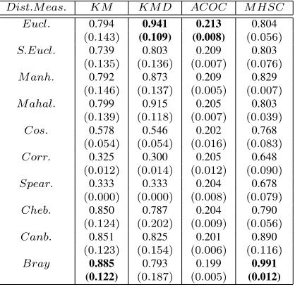
Dist.M eas. KM KM D ACOC M HSC Eucl. 0.794 0.941 0.213 0.804
(0.143) (0.109) (0.008) (0.056)
S.Eucl. 0.739 0.803 0.209 0.803
(0.135) (0.136) (0.007) (0.076)
M anh. 0.792 0.873 0.209 0.829
(0.146) (0.137) (0.005) (0.007)
M ahal. 0.799 0.915 0.205 0.803
(0.139) (0.118) (0.007) (0.039)
Cos. 0.578 0.546 0.202 0.768
(0.054) (0.054) (0.016) (0.083)
Corr. 0.325 0.300 0.205 0.648
(0.012) (0.014) (0.012) (0.090)
Spear. 0.333 0.333 0.204 0.678
(0.000) (0.000) (0.008) (0.079)
Cheb. 0.850 0.787 0.204 0.790
(0.124) (0.202) (0.009) (0.056)
Canb. 0.851 0.825 0.201 0.890
(0.123) (0.154) (0.006) (0.116)
Bray 0.885 0.793 0.199 0.991 (0.122) (0.187) (0.005) (0.012)
For Sph_6 _2 dataset (Table 15), K-Means pro-duces compact and accurate clusters with Bray-Curtis distance. A careful look at Figure 3(b) reveals that K-Means with Canberra distance provide well-separated clusters. From Figures 3(b) and 4(b), it has been seen
that K-Medoid with Euclidean distance gives well-separated and compact clusters having accuracy higher than the other distance measures. The ACOC technique with Euclidean distance attains better accuracy. How-ever, it produces well-separated and compact clusters with Mahalanobis and Cosine distance respectively. The MHSC with Bray-Curtis produces well-separated and compact clusters having higher accuracy when compared with other measures.
Table 16:Effect of distance measures on accuracy of cluster formed forSph_4_3dataset for Partitional Clustering Techniques
Dist.M eas. KM KM D ACOC M HSC Eucl. 0.909 0.957 0.286 0.973
(0.168) (0.121) (0.008) (0.077)
S.Eucl. 0.825 0.828 0.286 0.950
(0.187) (0.184) (0.008) (0.091)
M anh. 0.382 0.778 0.279 0.871
(0.025) (0.184) (0.007) (0.146)
M ahal. 0.520 0.526 0.278 0.771
(0.022) (0.018) (0.011) (0.143)
Cos. 0.413 0.415 0.270 0.702
(0.042) (0.055) (0.008) (0.139)
Corr. 0.301 0.295 0.269 0.710
(0.004) (0.004) (0.006) (0.109)
Spear. 0.293 0.295 0.272 0.657
(0.000) (0.000) (0.006) (0.164)
Cheb. 1.000 0.826 0.285 0.892
(0.000) (0.186) (0.007) (0.156)
Canb. 0.652 0.744 0.283 0.827
(0.217) (0.208) (0.009) (0.179)
Bray 0.604 0.818 0.288 0.656
(0.008) (0.077) (0.009) (0.081)
For Sph_4 _3 dataset (Table 16), K-Means with Chebychev distance offers highest accuracy over other distance measures. The K-Means with Chebychev distance generates well-separated and compact clus-ters. The K-Medoid provides better accuracy with compact clusters using Euclidean distance. While, it generates well-separated clusters using Bray-Curtis distance (Figure 3(c)). The ACOC technique with Bray-Curtis distance generates accurate, compact and well-separated clusters. The MHSC with Euclidean distance produces accurate, well-separated, and com-pact clusters as compared to other distance measures.
For Iris dataset, the K-Means clustering algorithm provides better accuracy with Chebychev distance. The K-Medoid technique with Manhattan distance attains best accuracy. Both K-Means and K-Medoid produce compact and well-separated clusters with Spearman distance. The ACOC with Spearman distance attains better accuracy. It produces compact clusters with
Table 17:Effect of distance measures on accuracy of cluster formed forIrisdataset for Partitional Clustering Techniques
Dist.M eas. KM KM D ACOC M HSC Eucl. 0.844 0.718 0.396 0.867
(0.131) (0.190) (0.013) (0.047)
S.Eucl. 0.844 0.713 0.392 0.882
(0.131) (0.196) (0.009) (0.068)
M anh. 0.767 0.841 0.395 0.885
(0.166) (0.133) (0.009) (0.055)
M ahal. 0.778 0.526 0.389 0.868
(0.036) (0.161) (0.021) (0.061)
Cos. 0.803 0.828 0.382 0.848
(0.235) (0.167) (0.011) (0.138)
Corr. 0.801 0.839 0.385 0.891
(0.221) (0.176) (0.008) (0.072)
Spear. 0.667 0.667 0.415 0.716
(0.000) (0.000) (0.033) (0.132)
Cheb. 0.887 0.768 0.385 0.871
(0.000) (0.174) (0.009) (0.032)
Canb. 0.867 0.774 0.366 0.883
(0.148) (0.191) (0.005) (0.067)
Bray 0.798 0.798 0.364 0.862
(0.165) (0.180) (0.007) (0.066)
Bray-Curtis and well-separated clusters with Canberra distance (Figures 3(d) and 4(d)). The MHSC technique provides well-separated and accurate clusters using Correlation distance. While, it offers compact clusters with Euclidean distance.
Table 18:Effect of distance measures on accuracy of cluster formed forW inedataset for Partitional Clustering Techniques
D.M eas. KM KM D ACOC M HSC Eucl. 0.669 0.631 0.432 0.691
(0.059) (0.080) (0.021) (0.054)
S.Eucl. 0.669 0.704 0.399 0.671
(0.059) (0.008) (0.015) (0.061)
M anh. 0.669 0.650 0.422 0.663
(0.066) (0.078) (0.028) (0.060)
M ahal. 0.609 0.459 0.368 0.638
(0.119) (0.036) (0.066) (0.059)
Cos. 0.685 0.657 0.409 0.689
(0.018) (0.000) (0.021) (0.048)
Corr. 0.685 0.669 0.415 0.665
(0.012) (0.013) (0.012) (0.058)
Spear. 0.664 0.608 0.389 0.655
(0.034) (0.088) (0.023) (0.073)
Cheb. 0.652 0.684 0.419 0.678
(0.069) (0.054) (0.021) (0.056)
Canb. 0.891 0.621 0.413 0.689
(0.129) (0.077) (0.008) (0.042)
Bray 0.717 0.719 0.419 0.678
(0.003) (0.007) (0.008) (0.072)
For Wine dataset, the K-Means technique attains higher accuracy with Canberra distance. It produces
well-separated clusters with Chebychev distance and compact clusters with Bray-Curtis distance (Figures 3(e) and 4(e)). K-Medoid attains optimal accuracy using Bray-Curtis distance. It gives well-separated clusters with Spearman distance and compact clusters with Mahalanobis distance. The ACOC technique with Euclidean distance provides better accuracy than the other measures. It provides compact clusters with Bray-Curtis and well-separated clusters with Canberra distance. The MHSC technique with Euclidean dis-tance offers accurate and well-separated clusters. It produces compact clusters with Cosine distance.
Table 19:Effect of distance measures on accuracy of cluster formed forGlassdataset for Partitional Clustering Techniques
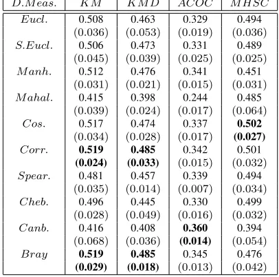
D.M eas. KM KM D ACOC M HSC Eucl. 0.508 0.463 0.329 0.494
(0.036) (0.053) (0.019) (0.036)
S.Eucl. 0.506 0.473 0.331 0.489
(0.045) (0.039) (0.025) (0.025)
M anh. 0.512 0.476 0.341 0.451
(0.031) (0.021) (0.015) (0.031)
M ahal. 0.415 0.398 0.244 0.485
(0.039) (0.024) (0.017) (0.064)
Cos. 0.517 0.474 0.337 0.502
(0.034) (0.028) (0.017) (0.027)
Corr. 0.519 0.485 0.342 0.501
(0.024) (0.033) (0.015) (0.032)
Spear. 0.481 0.457 0.339 0.494
(0.035) (0.014) (0.007) (0.034)
Cheb. 0.496 0.445 0.330 0.499
(0.028) (0.049) (0.016) (0.032)
Canb. 0.416 0.408 0.360 0.394
(0.068) (0.036) (0.014) (0.054)
Bray 0.519 0.485 0.345 0.476
(0.029) (0.018) (0.013) (0.042)
For Glass dataset, the K-Means and K-Medoid provides best accuracy with Correlation and Bray-Curtis distances. K-Means, K-Medoid, and ACOC techniques attain well-separated and compact clusters with Canberra distance (Figures 3(f) and 4(f)). ACOC technique provides good accuracy over Canberra distance. The MHSC technique gives accurate clusters with Cosine distance and well-separated clusters with Spearman distance. It produces compact clusters with Mahalanobis distance.
Kumar, Chhabra and Kumar Performance Evaluation of Distance Metrics in the Clustering Algorithms 49
Table 20:Effect of distance measures on accuracy of cluster formed forHabermandataset for Partitional Clustering Techniques
D.M eas. KM KM D ACOC M HSC Eucl. 0.509 0.594 0.672 0.554
(0.011) (0.104) (0.014) (0.040)
S.Eucl. 0.514 0.547 0.561 0.542
(0.008) (0.075) (0.015) (0.036)
M anh. 0.579 0.575 0.683 0.532
(0.107) (0.094) (0.014) (0.024)
M ahal. 0.522 0.546 0.523 0.548
(0.020) (0.085) (0.015) (0.033)
Cos. 0.513 0.536 0.713 0.583
(0.003) (0.016) (0.011) (0.087)
Corr. 0.509 0.531 0.711 0.558
(0.000) (0.018) (0.012) (0.062)
Spear. 0.647 0.664 0.647 0.581
(0.000) (0.006) (0.014) (0.078)
Cheb. 0.534 0.529 0.676 0.529
(0.011) (0.029) (0.011) (0.024)
Canb. 0.527 0.529 0.699 0.575
(0.001) (0.038) (0.010) (0.063)
Bray 0.509 0.550 0.724 0.534
(0.000) (0.087) (0.006) (0.027)
on Bray-Curtis distance. It generates well-separated clusters with Correlation and compact clusters with Spearman distance. The MHSC technique provides higher accuracy over cosine distance. It gives well-separated clusters with Spearman and compact clusters with City-Block distance (Figures 3(g) and 4(g)).
Table 21:Effect of distance measures on accuracy of cluster formed forBupadataset for Partitional Clustering Techniques
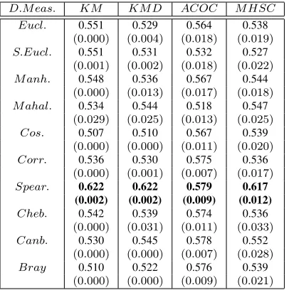
D.M eas. KM KM D ACOC M HSC Eucl. 0.551 0.529 0.564 0.538
(0.000) (0.004) (0.018) (0.019)
S.Eucl. 0.551 0.531 0.532 0.527
(0.001) (0.002) (0.018) (0.022)
M anh. 0.548 0.536 0.567 0.544
(0.000) (0.013) (0.017) (0.018)
M ahal. 0.534 0.544 0.518 0.547
(0.029) (0.025) (0.013) (0.025)
Cos. 0.507 0.510 0.567 0.539
(0.000) (0.000) (0.011) (0.020)
Corr. 0.536 0.530 0.575 0.536
(0.000) (0.001) (0.007) (0.017)
Spear. 0.622 0.622 0.579 0.617 (0.002) (0.002) (0.009) (0.012)
Cheb. 0.542 0.539 0.574 0.536
(0.000) (0.031) (0.011) (0.033)
Canb. 0.530 0.545 0.578 0.552
(0.000) (0.000) (0.007) (0.028)
Bray 0.510 0.522 0.576 0.539
(0.000) (0.000) (0.009) (0.021)
For the Bupa dataset (Table 21), Means,
K-Medoid, and ACOC produces accurate clusters with compactness using Spearman distance. K-Means gives well-separated clusters using Standard Euclidean dis-tance. K-Medoid and ACOC generate well-separated clusters with Spearman and Bray-Curtis distances respectively. The MHSC algorithm provides better accuracy with Spearman distance. It gives compact clusters with Canberra and well-separated clusters with Cosine distance (Figures 3(h) and 4(h)).
Table 22:Effect of distance measures on accuracy of cluster formed forLibrasdataset for Partitional Clustering Techniques
D.M eas. KM KM D ACOC M HSC Eucl. 0.188 0.191 0.071 0.157
(0.048) (0.048) (0.007) (0.044)
S.Eucl. 0.207 0.134 0.064 0.159
(0.065) (0.094) (0.013) (0.048)
M anh. 0.175 0.151 0.079 0.140
(0.070) (0.062) (0.009) (0.058)
M ahal. 0.084 0.066 0.063 0.145
(0.028) (0.009) (0.004) (0.039)
Cos. 0.235 0.198 0.074 0.155
(0.079) (0.044) (0.011) (0.049)
Corr. 0.259 0.182 0.075 0.159
(0.049) (0.047) (0.007) (0.062)
Spear. 0.224 0.117 0.078 0.152
(0.037) (0.051) (0.007) (0.029)
Cheb. 0.248 0.186 0.078 0.121
(0.064) (0.037) (0.011) (0.046)
Canb. 0.183 0.178 0.078 0.147
(0.052) (0.060) (0.007) (0.052)
Bray 0.175 0.182 0.071 0.193
(0.059) (0.094) (0.009) (0.047)
ForLibrasdataset results given in Table 22, show that the K-Means using Correlation distance attains best accuracy. However, it gives compact clusters with Bray-Curtis and well-separated clusters with Canberra distance. K-Medoid provides accurate clusters on Co-sine distance and compact clusters with Mahalanobis. It generates well-separated clusters with Euclidean dis-tance. ACOC provides accurate clusters on Manhattan distance and compact clusters with Chebyshev. How-ever, it generates well-separated clusters with Spearman distance. The MHSC technique attains high accuracy over Bray-Curtis distance. It gives well-separated and compact clusters with City-Block distance (Figures 3(i) and 4(i)).
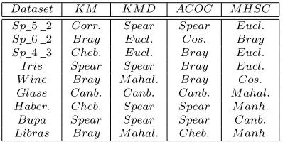
The aforementioned results indicate that the different distance measures with clustering techniques show dif-ferent cluster quality value. The summarized results for partitional techniques are tabulated in Tables 23, 24 and 25.
Table 23:Best distance measures corresponding to datasets and par-titional clustering techniques in terms of Accuracy
Dataset KM KM D ACOC M HSC Sp_5_2 Cheb. Eucl. Bray. Eucl. Sp_6_2 Bray Eucl. Eucl. Bray Sp_4_3 Eucl. Eucl. Bray Eucl. Iris Cheb. M ahal. Spear Corr. W ine Canb. Bray Eucl. Eucl. Glass Corr. Corr. Canb. Cos.
Bray Bray
Haber. Spear Spear Bray Cos. Bupa Spear Spear Spear Spear Libras Corr. Cos. M anh. Bray
Table 24:Best distance measures corresponding to datasets and par-titional clustering techniques in terms of Inter-cluster Distance
Dataset KM KM D ACOC M HSC Sp_5_2 Spear Spear Spear Canb. Sp_6_2 Canb. Eucl. M ahal. Bray Sp_4_3 Cheb. Bray Bray Eucl. Iris Spear Spear Canb. Corr. W ine Cheb. Spear Canb. Eucl. Glass Canb. Canb. Canb. Spear Haber. Spear Spear Corr. Spear Bupa S.Eucl. Spear Bray Cos. Libras Canb. Eucl. Spear M anh.
Table 25:Best distance measures corresponding to datasets and par-titional clustering techniques in terms of Intra-cluster Distance
Dataset KM KM D ACOC M HSC Sp_5_2 Corr. Spear Spear Eucl. Sp_6_2 Bray Eucl. Cos. Bray Sp_4_3 Cheb. Eucl. Bray Eucl. Iris Spear Spear Bray Eucl. W ine Bray M ahal. Bray Cos. Glass Canb. Canb. Canb. M ahal. Haber. Cheb. Spear Spear M anh. Bupa Spear Spear Spear Canb. Libras Bray M ahal. Cheb. M anh.
5 Conclusion
In this paper, performance of ten commonly used dis-tance measures in clustering techniques has been eval-uated. The eight well-known clustering algorithms are evaluated on ten different datasets. The experimental results are evaluated in terms of accuracy, inter-cluster and intra-cluster distances. It has been observed that there is no single best distance measure for all datasets, or for all quality measures. The appropriateness of a distance measure is dependent on nature of data and clustering technique. On basis of our experimentation, we have reported a set of suitable distance measures
for a particular combination of distance and clustering techniques.
References
[1] Bandyopadhyay, S. and Maulik, U. Genetic clus-tering for automatic evolution of clusters and ap-plication to image classification.Pattern Recogni-tion, 35(6):1197–1208, 2002.
[2] Bray, J. R. and Curtis, J. T. An ordination of the upland forest communities of southern wisconsin.
Ecological Monographs, 27(4):325–349, 1957.
[3] Cao, F., Liang, J., Li, D., Bai, L., and Dang, C. A dissimilarty measure for the k-modes clustering algorithm.Knowledge-Based Systems, 26(1):120– 127, 2012.
[4] Chen, J., Zhao, Z., Ye, J., and Liu, H. Nonlin-ear adaptive distance metric lNonlin-earning for cluster-ing. InProceedings of International Conference on Knowledge Discovery and Data Mining, pages 123–132, 2007.
[5] Fulekar, M. H. Bioinformatics: Applications in Life and Environmental Sciences. Springer, 2009.
[6] Huang, A. Similarity measures for text docu-ment clustering. InProceedings of the Sixth New Zealand Computer Research Student Conference, pages 49–56, 2008.
[7] Jain, A. K. and Dubes, R. C. Algorithms for Clustering Data. Prentice Hall, Englewood Cliffs, 1988.
[8] Kaufman, L. and Rousseeuw, P. J.Finding groups in data: an introduction to cluster analysis. John Wiley and Sons, New York, 1990.
[9] Kumar, V., Chhabra, J. K., and Kumar, D. Effect of harmony serach parameters’ variation in clus-tering.Procedia Technology, 6:265–274, 2012.
[10] Kumar, V., Chhabra, J. K., and Kumar, D. Cluster-ing usCluster-ing modified harmony search algorithm. In-ternational Journal of Computational Intelligence Studies, 3(2):113–133, 2014.
[11] Lance, G. N. and Williams, W. T. Computer programs for hierarchical polythetic classifica-tion (similarity analyses). Computer, 9(1):60–64, 1966.
Kumar, Chhabra and Kumar Performance Evaluation of Distance Metrics in the Clustering Algorithms 51
[13] Maulik, U. and Bandyopadhyay, S. Performance evaluation of some clustering algorithms and va-lidity indices.IEEE Transactions on Pattern Anal-ysis and Machine Intelligence, 24(12):1650–1654, 2002.
[14] Newman, C. L., Blake, D., and Merz, C. J. Uci repository of machine learning databases, 1998.
[15] Potolea, R., Cacoveanu, S., and Lemnaru, C. Meta-learning framework for prediction strategy evaluation. InProceedings of International Con-ference on Enterprise Information Systems, pages 280–295, Magdeburg, Germany, 2011.
[16] Prekopcsak, Z. and Lemire, D. Time series clas-sification by class-specific mahalanobis distance measures.Advances in Data Analysis and Classi-fication, 2(1):49–55, 2012.
[17] Shelokar, P. S., Jayaraman, V. K., and Kulkarni, B. D. An ant colony approach for clustering. An-alytica Chimica Acta, 509(2):187–195, 2004.
[18] Tan, P. N., Steinbach, M., and Kumar, V. Intro-duction to data mining. Addison-Wesley, 2005.
[19] Vadapalli, S. on the ignored aspects of data clus-tering. InGHC of Women in Computing, pages 6–10, 2004.
[20] Vimal, A., Valluri, S., and Karlapalem, K. An experiment with distance measures for clustering. Technical Report IIIT/TR/2008/132, Center for Data Engineering, IIIT, Hyderabad, July 2008.
[21] Xu, R. and Wunsch, D. Survey of clustering algo-rithms. IEEE Transactions on Neural Networks, 16(3):120–127, 2005.