www.theoryofcomputing.org
S
PECIAL ISSUE: APPROX-RANDOM 2015
A Randomized Online Quantile Summary
in
O((
1/
ε
)
log
(
1/
ε
))
Words
David Felber
Rafail Ostrovsky
∗Received November 18, 2015; Revised May 16, 2017; Published November 14, 2017
Abstract: A quantile summary is a data structure that approximates toε error the order
statistics of a much larger underlying dataset.
In this paper we develop a randomized online quantile summary for the cash register data input model and comparison data domain model that uses O((1/ε)log(1/ε))words
of memory. This improves upon the previous best upper bound ofO((1/ε)log3/2(1/ε))by
Agarwal et al. (PODS 2012). Further, by a lower bound of Hung and Ting (FAW 2010) no deterministic summary for the comparison model can outperform our randomized summary in terms of space complexity. Lastly, our summary has the nice property thatO((1/ε)log(1/ε))
words suffice to ensure that the success probability is at least 1−exp(−poly(1/ε)).
ACM Classification:F.2.2, E.1, F.1.2
AMS Classification:68W20, 68W25, 68W27, 68P05
Key words and phrases:algorithms, data structures, data stream, approximation, approximation
algo-rithms, online algoalgo-rithms, randomized, summary, quantiles, RANDOM
A conference version of this paper appeared in theProceedings of the 19th Internat. Workshop on Randomization and Computation (RANDOM 2015).
∗Research supported in part by NSF grants CCF-0916574; IIS-1065276; CCF-1016540; CNS-1118126; CNS-1136174;
1
Introduction
A quantile summarySis a fundamental data structure that summarizes an underlying datasetXof sizen, in space much less thann. Given a queryφ,Sreturns an elementyofX such that the rank ofyinXis
(probably) approximatelyφn. Quantile summaries are used in sensor networks to aggregate data in an
energy-efficient manner and in database query optimizers to generate query execution plans.
1.1 The model
Quantile summaries have been developed for a variety of different models and metrics. The data input model we consider is the standard online cash register streaming model. In this model there is a single machine at which computation takes place. Attached to the machine is a data stream that feeds items to the machine one at a time online. Time is measured in stream items received, so that the first itemx1 arrives att=1, the second at timet=2, and so forth. After eachxt arrives, the machine may do any processing that it needs to do. Timesteptdoes not end, and timet+1 does not start, until this processing is complete. The set of all stream items received through timetis denotedXt orX(t). Xt can also be viewed as a (multi)set of thet-item prefix of the infinite streamXof all stream items that will be fed to the machine. In addition to receiving the data stream, the machine is also able to accept and answer queries. After stream itemxt arrives, the machine can be given queriesφ, to which it responds within the same timestept. The next itemxt+1does not arrive until any queries for timestepthave completed. Further, for randomized algorithms, the machine has a source of randomness from which it can sample random bits. The data domain model we consider is the comparison model, in which stream items come from an arbitrary totally ordered domainDof stream items. Dis specifically not required to be the integers. Stream items are indivisible tokens. The only operations permitted on stream items is to compare them and to copy, move, and delete them. In particular, stream items do not need to have any numeric value, and the comparison function can be an arbitrarily complex one.
The memory model we consider has two regions of memory. The first region can contain only stream items. Each copy of a stream item uses one unit of memory. When a new stream itemxt arrives from the data stream it arrives at a set location in this region of memory, and during processing can be copied to other locations in this region. When the next stream itemxt+1arrives, ifxt was not copied, thenxt+1 overwrites the only copy ofxt, and thereforext is lost and cannot be retrieved. Stream items can also be deleted from this region, in which case they are also lost and cannot be retrieved.
The second region of memory is a scratch pad or bookkeeping area that can store numeric tokens and perform operations with and on those tokens. In particular, the operations permitted on the tokens are arithmetic, comparison, referencing locations of stream items in the first region of memory, and referencing locations of numeric tokens in the second region of memory. Also, to support randomness, the machine can in one operation sample a random bit into a fixed numeric token location in this second memory region. Each numeric token can take on a value in{0,1,2, . . . ,max}, where max isO(t)for a constant number of those tokens andO(poly(1/ε))for the rest of the tokens.
1.2 The problem
Our problem is defined by an error parameterε≤1/2. The goal is to maintain in the machine at all times
ta quantile summarySt of the datasetXt. A quantile summary is a data structure with two operations. The first is an update operation, that takes a summarySt−1and a stream itemxt and returns an updated summarySt. This update operation is performed in the processing phase of each timestep after stream itemxt arrives. The second operation is a query operation, that takes a summarySt and a valueφ in (0,1], and returns a stream itemy=y(φ)from the first memory region (and therefore fromXt) so that |R(y,Xt)−φt| ≤εt, whereR(a,Z)is therank of item a in set Z, defined as|{z∈Z:z≤a}|.
For randomized quantile summaries, there is an additional parameterδ, and we only require that for
any timetand any queryφwe have thatP(|R(y,Xt)−φt| ≤εt) ≥1−δ; that is,y’s rank is only probably close toφt, not definitely close. For our main result we use a fixedδ =e−poly(1/ε). It will be easier to
deal with the rank directly, so we defineρ=φtand use that in what follows.
In either case, the measure of an algorithm for the problem is the space required to store the quantile summary, meaning that the number of stream items should be small and also the number of numeric tokens should be small. The algorithm we develop here uses O((1/ε)log(1/ε)) stream items and
O((1/ε)log(1/ε))numeric tokens through timet. Calling each of these stream items or numeric tokens
a memory word, our algorithm uses a total ofO((1/ε)log(1/ε))words.
The quantile summary is maintained in memory. Any stream items in the data structure are stored in the first memory region that contains only stream items. Any bookkeeping information, such as the numbert, is stored in the second memory region. However, to make our algorithm easy to understand we ignore this distinction in the algorithm’s description.
Lastly, note that the problem of maintaining a small summary is only interesting in the online case, in which items arrive one by one. Offline, a trivial summary ofXn is the set of 1/ε items at ranks
εn,2εn,3εn, . . . ,n.
1.3 Previous and related work
The two most directly relevant pieces of prior work ([1] and [8]) are randomized online quantile summaries for the cash register/comparison model. Aside from oblivious sampling algorithms (which require storing
Ω(1/ε2)samples) the only other such work of which we are aware is an approach by Wang, Luo, Yi, and
Cormode [12] that combines the methods of [1] and [8] into a hybrid with the same space bound as [1]. The newer of the two is that of Agarwal, Cormode, Huang, Phillips, Wei, and Yi [1]. Among other results, Agarwal et al. develop a randomized online quantile summary for the cash register/comparison model that usesO((1/ε)log3/2(1/ε))words of memory. This summary has the nice property that any
two such summaries can be combined to form a summary of the combined underlying dataset without loss of accuracy or increase in size.
The earlier such summary is that of Manku, Rajagopalan, and Lindsay [8], which uses(1/ε)log2(1/ε)
space. At a high level, their algorithm downsamples the input stream in a non-uniform way and feeds the downsampled stream into a deterministic summary, while periodically adjusting the downsampling rate.
For the comparison model, the best deterministic online summary to date is the (GK) summary of Greenwald and Khanna [4], which usesO((1/ε)log(εn))space. This improved upon a deterministic (MRL) summary of Manku, Rajagopalan, and Lindsay [7] and a summary implied by Munro and Paterson [9], which useO((1/ε)log2(εn))space.
A more restrictive domain model than the comparison model is the bounded universe model, in which elements are drawn from the integers{1, . . . ,u}. For this model there is a deterministic online summary by Shrivastava, Buragohain, Agrawal, and Suri [10] that usesO((1/ε)log(u))space.
Between submission of our paper to Theory of Computing and its acceptance, a new method was developed by Karnin, Lang, and Liberty [6] that obtains matching upper and lower bounds for the problem of maintaining a randomized online summary. Their upper bound,O((1/ε)log log(1/δ)), can be viewed as extending our upper bound ofO((1/ε)log(1/ε))to arbitraryδ, which is particularly valuable whenδ
is large compared to e−poly(1/ε). Prior to [6] the best lower bound was a simple lower bound of
Ω(1/ε)
which intuitively comes from the fact that no one element can satisfy more than 2εndifferent rank queries. For the deterministic version of the problem there is a lower bound ofΩ((1/ε)log(1/ε))by Hung and
Ting [5].
1.4 Our contributions
In the next section we describe a simpleO((1/ε)log(1/ε))streaming summary that is online except
that it requiresnto be given up front and that it is unable to process queries until it has seen a constant fraction of the input stream. This simple summary is not new (it is mentioned in Wang et al. [12], for example) but the discussion provides exposition forSection 3, in which we develop this summary into a fully online summary with the same asymptotic space complexity that can answer queries at any point in time. At that point we will have proven the following theorem, which constitutes our main result.
Theorem 1.1. There is a randomized online quantile summary algorithm that runs in deterministic
O((1/ε)log(1/ε))space and guarantees that, for any sequence X of items, for any n, and for any rank
ρ≤n, the summary’s response to queryρ just after receiving xnwill be an item y∈Xnsuch that
P(|R(y,Xn)−ρ| ≤εn) ≥1−exp(−1/ε).
Finally, we close inSection 4by examining the similarities and differences between our summary and previous work and discuss a design approach for similar streaming problems.
2
A simple streaming summary
Before we describe the algorithm we must first describe its two main components in a bit more detail than was used in the introduction. The two components are Bernoulli sampling and the GK summary [4].
2.1 Bernoulli sampling
advance.) At the end of processingX, the expected size ofSism, and the expected rank of any sampleyin SisE(R(y,S)) = (m/n)R(y,X). In fact, for any timest≤nand partial streamsXt andSt, whereSt is the sample stream ofXt, we haveE(|St|) =mt/nandE(R(y,St)) = (m/n)R(y,Xt). To generate an estimate forR(y,Xt)fromSt we use ˆR(y,Xt) = (n/m)R(y,St). The following theorem bounds the probability that Sis very large or that ˆR(y,Xt)is very far fromR(y,Xt). A generalization of this theorem is due to Vapnik and Chervonenkis [11]; the proof of this special case is a simple known application of Chernoff bounds.
Theorem 2.1. Let0≤m≤n and0<ε <1. For any time t≥n/64,
P(|St|>2tm/n) <exp(−m/192).
Further, for any time t≥n/64and any item y,
P(|Rˆ(y,Xt)−R(y,Xt)|>εt/8) <2 exp(−ε2m/12288).
Proof. For the first part we use a Chernoff bound of
P(|St|>(1+δ)E(|St|))<exp(−δE(|St|)/3).
Here,E(|St|) =tm/n, soδ =1, and
P(|St|>2tm/n) <exp(−tm/3n) <exp(−m/192)
sincet≥n/64. For the second part,
P(|Rˆ(y,Xt)−R(y,Xt)|>εt/8) =P(|R(y,St)−E(R(y,St))|>εtm/8n).
The Chernoff bound is
P(|R(y,St)−E(R(y,St))|>δE(R(y,St)))<2 exp(−min{δ,δ2}E(R(y,St))/3). Here,δ =εt/8E(R(y,St)). Ifδ2>δ>1 then
P <2 exp(−εt/24)≤ 2 exp(−εn/1536)≤ 2 exp(−ε2m/12288).
Otherwise,δ2≤δ≤1, in which case
P <2 exp(−ε2t2m/192nE(R(y,St)))≤2 exp(−ε2m/12288), finishing the proof.
This means that, given any 1≤ρ≤t, if we choose to return the sampley∈St withR(y,St) =ρm/n, thenR(y,Xt)is likely to be close toρ, as long asmisΩ((1/ε2)log(1/ε))
2.2 GK summary
The GK summary is a deterministic summary that can answer queries toε error over any portion of
2.3 A simple streaming summary
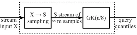
We combine Bernoulli sampling with the GK summary by downsampling the input data streamX to a sample streamSand then feedingSinto a GK summaryG. It looks like this.
X → S
sampling ≈ m samples GK(ε/8)S stream of stream
input X quantilesquery
Figure 1: The big picture.
The key reason this gives us a small summary is that we never need to storeS; each time we sample an item intoSwe immediately feed it intoG. Therefore, we only use as much space asG(S(Xt))uses. In particular, form=O(poly(1/ε)), we use onlyO((1/ε)log(1/ε))words. To answer a queryρforXt, we scaleρ bym/n, askG(S(Xt))for that, and return the resulting sampley.
We formalize this intuition in the following lemma, which combines the ideas in the proof of Theorem 2.1with the GK guarantee to yield approximation and correctness guarantees.
Lemma 2.2. Fix some time t≥n/64 and some rank ρ ≤t, and consider querying G(S(Xt)) with
q=min{ρm/n,|S|}, obtaining y as the result. Say that S=S(Xt)isgoodif
|S| −mt/n
≤εmt/8n
and if none of the first≤mt/n samples z in S has
R(z,S)−
m
nR(z,Xt)
>εmt/8n.
If S is good then
|R(y,Xt)−ρ| ≤εt/2. Further, if
m≥400000 ln 1/ε
ε3
then
P(S is not good)≤ε3e−1/ε/8.
Proof. First, by the GK guarantee,G(S)returns some itemywith|R(y,S)−q| ≤εt/8. IfSis good, then
q−
ρm
n
≤
εmt
8n , and also
R(y,S)−
m
nR(y,Xt)
≤
εmt
8n . By the triangle inequality,
m
nR(y,Xt)−
ρm n
≤
Now, following the proof ofTheorem 2.1, we have that
P(||St| −mt/n|>εmt/8n)< 2 exp(−ε2m/12288)
and also for each of the first≤msampleszthat
P(|R(z,S)−mnR(z,Xt)|>εmt/8n)<2 exp(−ε2m/12288).
By the union bound,
P(Sis not good)≤4mexp(−ε2m/12288).
Choosing
m≥400000 ln 1/ε
ε3
suffices to bound this quantity byε3e−1/ε/8.
2.4 Caveats
There are two serious issues with this summary. The first is that it requires us to know the value ofnin advance to perform the sampling. Also, as a byproduct of the sampling, we can only obtain approximation guarantees after we have seen at least 1/64 (or at least some constant fraction) of the items. This means that while the algorithm is sufficient for approximating order statistics over streams stored on disk, more is needed to get it to work for online streaming applications, in which (1) the stream sizenis not known in advance, and (2) queries can be answered approximately at any timet≤nand not just whent≥n/64. Adapting this basic streaming summary idea to work online constitutes the next section and the bulk of our contribution. We start with a high-level overview of our online summary algorithm. In Section 3.1we formally define an initial version of our algorithm whose expected size at any given time is O((1/ε)log(1/ε))words. InSection 3.2we show that our algorithm guarantees that for anynand anyρ
we have thatP(|R(y,Xn)−ρ| ≤εn) ≥1−exp(−1/ε). InSection 3.3we discuss the slight modifications
necessary to get a deterministicO((1/ε)log(1/ε))space complexity, and also perform a time complexity
analysis.
3
An online summary
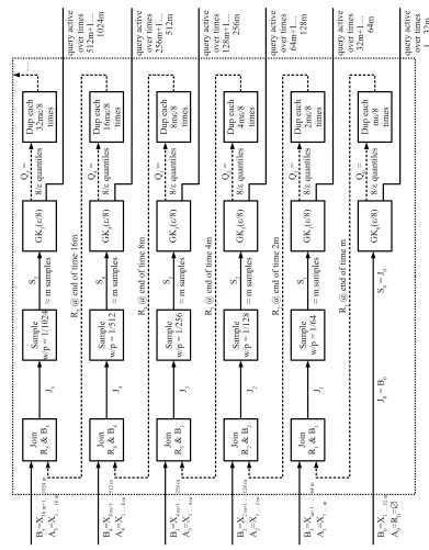
Our algorithm works inrows, which are illustrated inFigure 2andFigure 3. Rowr is a summary of the first 2r32mstream items. Since we do not know how many items will actually be in the stream, we cannot start all of these rows running at the outset. Therefore, we start each rowr≥1 once we have seen 1/64 of its total items. However, since we cannot save these items for every row we start, we need to construct an approximation of this fraction of the stream, which we do by using the summary of the previous row, and join this approximating stream with the new items that arrive while the row is live. We then wait until the row has seen a full half of its items before we permit it to start answering queries; this dilutes the influence of approximating the 1/64 of its input that we could not store.
G K0 (ε/ 8) D up e ac h m ε/ 8 tim es G K1 (ε/ 8) D up e ac h 2m ε/ 8 tim es Sa m pl e w /p = 1 /64 Jo in R1 & B1 J1 S1 ≈ m s am pl es Q1 = 8/ ε qua nt ile s Q0 = 8/ ε qua nt ile s R1 @ e nd of ti m e m G K2 (ε/ 8) D up e ac h 4m ε/ 8 tim es Sa m pl e w /p = 1 /12 8 Jo in R2 & B2 J2 S2 ≈ m s am pl es Q2 = 8/ ε qua nt ile s R2 @ e nd of ti m e 2m G K3 (ε/ 8) D up e ac h 8m ε/ 8 tim es Sa m pl e w /p = 1 /25 6 Jo in R3 & B3 J3 S3 ≈ m s am pl es Q3 = 8/ ε qua nt ile s R3 @ e nd of ti m e 4m G K4 (ε/ 8) D up e ac h 16 m ε/ 8 tim es Sa m pl e w /p = 1 /51 2 Jo in R4 & B4 J4 S4 ≈ m s am pl es Q4 = 8/ ε qua nt ile s R4 @ e nd of ti m e 8m R5 @ e nd o f t im e 16 m B0 = X1 … 3 2 m A0 = R0 = ∅ B1 = Xm +1 … 64 m A1 = X1 … m B2 = X2 m +1 … 128 m A2 = X1 … 2 m B3 = X4 m +1 … 256 m A3 = X1 … 4 m B4 = X8 m +1 … 512 m A4 = X1 … 8 m qu er y a ct iv e ov er ti m es 1…32m qu er y a ct iv e ov er ti m es 32m + 1… 64m qu er y a ct iv e ov er ti m es 64m + 1… 128m qu er y a ct iv e ov er ti m es 128m + 1… 256m qu er y a ct iv e ov er ti m es 256m + 1… 512m J0 = B0 G K5 (ε/ 8) D up e ac h 32 m ε/ 8 tim es Sa m pl e w /p = 1/ 10 24 Jo in R5 & B5 J5 S5 ≈ m s am pl es Q5 = 8/ ε qua nt ile s B5 = X16 m +1… 102 4 m A5 = X1 … 16 m qu er y a ct iv e ov er ti m es 512m + 1… 1024 m … S0 = J0
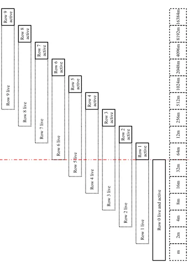
m 2m 4m 8m 16m 32m 64m 12m 256m 512m 1024 m 2048 m 4096 m 8192 m 16 384 m R ow 0 l iv e a nd a ct ive R ow 1 l iv e R ow 1 ac ti ve R ow 2 l iv e R ow 2 ac ti ve R ow 3 l iv e R ow 3 ac ti ve R ow 4 l iv e R ow 4 ac ti ve R ow 5 l iv e R ow 5 ac ti ve R ow 6 l iv e R ow 6 ac ti ve R ow 7 l iv e R ow 7 ac ti ve R ow 8 l iv e R ow 8 ac ti ve R ow 9 l iv e R ow 9 ac ti ve
Figure 3: There are at most six live rows and one active row at any time. Time is shown here in dashed boxes at the bottom of the diagram on a logarithmic scale; for example, box 2mrepresents items
is then fed into a GK summary (which is stored). After rowrhas seen half of its items, its GK summary becomes the one used to answer quantile queries. When rowr+1 has seen 1/64 ofitstotal items, rowr generates an approximation of those items from its GK summary and feeds them as a stream into row
r+1.
Row 0 is slightly different in order to bootstrap the algorithm. There is no join step since there is no previous row to join. Also, row 0 is active from the start. Lastly, we get rid of the sampling step so that we can answer queries over timesteps 1, . . . ,m/2.
After the first 32mitems, row 0 is no longer needed, so we can clean up the space used by its GK summary. Similarly, after the first 2r32mitems, rowris no longer needed. The upshot of this is that we never need storage for more than six rows at a time. Since each GK summary usesO((1/ε)log(1/ε))
words, the six live GK summaries also only useO((1/ε)log(1/ε))words.
Our error analysis, on the other hand, will require us to look back as many asΘ(log 1/ε)rows to
ensure our approximation guarantee. We stress that we will not need to actuallystoretheseΘ(log 1/ε)
rows for our guarantee to hold; we will only need that they did not have any bad events (as will be defined) when theywerealive.
3.1 Algorithm description
Our algorithm works in rows. Each rowrhas its own copyGrof the GK algorithm that approximates its input toε/8 error. For each rowrwe define several streams: Aris the prefix stream of rowr,Bris its suffix stream,Rris its prefix stream replacement (generated by the previous row),Jris the joint streamRr followed byBr,Sris its sample stream, andQris a one-time stream generated fromGrby querying it with ranksρ1, . . . ,ρ8/ε, whereρq=q(ε/8)(m/32)forr≥1 andρq=qεm/8 forr=0.
The prefix streamAr=X(2r−1m)for rowr≥1, importantly, is not directly received by rowr. Instead, at the end of timestep 2r−1m, rowr−1 generatesQr−1and duplicates each of those 8/εitems 2r−1εm/8
times to get the replacement prefixRr, which is then immediately fed into rowrbefore timestep 2r−1m+1 begins.
Each row can beliveor not andactiveor not. Row 0 is live in timesteps 1, . . . ,32mand rowr≥1 is live in timesteps 2r−1m+1, . . . ,2r32m. Live rows require space; once a row is no longer live we can free up the space it used. Row 0 is active in timesteps 1, . . . ,32mand rowr≥1 is active in timesteps
2r16m+1, . . . ,2r32m. This definition means that exactly one rowr(t)is active in any given timestept.
Any queries that are asked in timesteptare answered byGr(t). Given queryρ, we askGr(t)forρ/2r(t)32
(ifr≥1) or forρ(ifr=0) and return the result.
At each timestept, when itemxt arrives, it is fed as the next item in the suffix streamBrfor each live rowr.Brjoined withRrdefines the joined input streamJr. Forr≥1,Jris downsampled to the sample streamSrby sampling each item independently with probability 1/2r32. For row 0, no downsampling is performed, soS0=J0. Lastly,Sris fed intoGr.
Initially, allocate space forG0. Mark row 0 as live and active.
fort=1,2, . . .do
foreachlive row r≥0do
with probability1/2r32do
Insertxt intoGr.
ift=2r−1m for some r≥1then
Allocate space forGr. Mark rowras live. QueryGr−1withρ1, . . . ,ρ8/ε to gety1, . . . ,y8/ε.
forq=1, . . . ,8/εdo
for1, . . . ,2r−1εm/8do
with probability1/2r32do
InsertyqintoGr.
ift=2r16m for some r≥1then
Unmark rowr−1 as active and mark rowras active. Unmark rowr−1 as live and free space forGr−1.
onqueryρdo
Letr=r(t)be the active row.
QueryGrfor rankρ/2r32 (ifr≥1) or for rankρ (ifr=0). Return the result.
Algorithm 1:Procedural listing of the algorithm inSection 3.1.
3.2 Error analysis
DefineCr=x(2r32m+1),x(2r32m+2), . . .andYrto beRrfollowed byBrand thenCr. That is,Yris just the continuation ofJrfor the entire length of the input stream.
Fix some timet. All of our claims will be relative to timet; that is, if we writeSrwe meanSr(t). Our error analysis proceeds as follows. We start by proving thatR(y,Yr)is a good approximation ofR(y,Yr−1) when certain conditions hold forSr−1. By induction, this means thatR(y,Yr)is a good approximation of R(y,X=Y0)when the conditions hold for all ofS0, . . . ,Sr−1, and actually it is enough for the conditions to hold for justSr−log 1/ε, . . . ,Sr−1 to get a good approximation. Having proven this claim, we then
prove that the resulty=y(ρ) of a query to our summary has R(y,X) close to ρ. Lastly, we show
thatm=O(poly(1/ε))suffices to ensure that the conditions hold forSr−log 1/ε, . . . ,Sr−1with very high
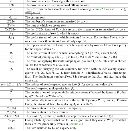
probability (1−e−1/ε).Table 1summarizes the quantities used in this and the preceding section.
Lemma 3.1. Letαrbe the event that|Sr|>2m and letβrbe the event that any of the first≤2m samples
z in Srhas
|2r32R(z,Sr)−R(z,Yr)|>
εt
8 .
Say that Srisgoodif neitherαrnorβroccur (or if r=0). For all rows r≥1such that t≥tr=2r−1m,
and all for all items y, if Sr−1is good then we have that
Proof. At the end of timetrwe haveYr(tr) =Rr(tr), which is each itemy(ρq)inQr−1duplicatedεtr/8 times. IfSr−1(tr)is good then|R(y(ρq),Yr−1(tr))−2r−132ρq| ≤εtr/2 followingLemma 2.2.
Fix q so that y(ρq)≤y<y(ρq+1), where y(ρ0) and y(ρ1+8/ε) are defined to be infD and supD
for completeness. Fixing q this way implies that R(y,Yr(tr)) =2r−132ρq. By the above bound on R(y(ρq),Yr−1(tr))we also have that
2r−132ρq−εtr/2 ≤R(y,Yr−1(tr))<2r−132ρq+1+εtr/2.
Recalling thatρq=qεm/256, these bounds imply that
|R(y,Yr(tr))−R(y,Yr−1(tr))| ≤2rεm.
For each timetaftertr, the new itemxt changes the rank ofyin both streamsYrandYr−1by the same additive offset, so
|R(y,Yr)−R(y,Yr−1)|=|R(y,Yr(tr))−R(y,Yr−1(tr))| ≤ 2rεm,
yielding the lemma.
By applying this lemma inductively we can bound the difference betweenYrandX=Y0as follows.
Corollary 3.2. For any r≥1such that t≥tr=2r−1m, if all of S0(t1),S1(t2), . . . ,Sr−1(tr)are good, then
|R(y,Yr)−R(y,X)| ≤2·2rεm.
To ensure that all of theseSiare good would requiremto grow withn, which would be bad, because the space complexity would also need to grow withn. Happily, it is enough to require only the last log21/ε sample summaries to be good, since the other items we disregard constitute only a small fraction
of the total stream.
Corollary 3.3.Let d=log21/ε. For any r≥1such that t≥tr=2r−1m, if all of Sr−1(tr), . . . ,Sr−d(tr−d+1)
are good, then|R(y,Yr)−R(y,X)| ≤2r+2εm.
Proof. ByLemma 3.1we have|R(y,Yr)−R(y,Yr−d)| ≤2r+1εm. At timet≥tr−d,Yr−dandXshare all
except possibly the first 2(r−d)−1m=2r−1m/2d=2r−1εmitems. Thus
|R(y,Yr)−R(y,X)| ≤ |R(y,Yr)−R(y,Yr−d)|+|R(y,Yr−d)−R(y,X)| ≤2r+1εm+2rεm,
proving the corollary.
We now prove that if the last several sample streams were good then querying our summary will give us a good result.
Lemma 3.4. Let d=log2(1/ε)<– and r=r(t). If all Sr(t),Sr−1(tr), . . . ,Sr−d(tr−d+1)are good, then
querying our summary with rankρ(= querying the active GK summary Grwithρ/2r32if r≥1, or with
Proof. For r ≥1 we have by Corollary 3.3 that |R(y,Yr)−R(y,X)| ≤2r+2εm≤εt/2. We apply
Lemma 2.2once more at rowr, which tells us that|R(y,Yr)−ρ| ≤εt/2, and combine these bounds with the triangle inequality.
Forr=0, the GK guarantee alone proves the lemma.
Lastly, we prove thatm=O(poly(1/ε))suffices to ensure that all ofSr(t),Sr−1(tr), . . . ,Sr−d(tr−d+1) are good with probability at least 1−e−1/ε.
Lemma 3.5. Let d=log21/ε and r=r(t). If
m≥400000 ln 1/ε
ε3
then all of Sr(t),Sr−1(tr), . . . ,Sr−d(tr−d+1)are good with probability at least1−e−1/ε.
Proof. There are at most 1+log21/ε≤4/ε of these summary streams total.Lemma 2.2and the union
bound give us
P(someSris bad) ≤ 4
ε ε3
8 e
−1/ε ≤e−1/ε,
which implies our claim.
3.3 Space and time complexity
A minor issue with the algorithm is that, as written inSection 3.1, we do not actually have a bound on the worst-case space complexity of the algorithm; we only have a bound on the space needed at any given point in time. This issue is due to the fact that there are low probability events in which|Sr|can get arbitrarily large and the fact that overnitems there are a total ofΘ(logn)sample streams. The space
complexity of the algorithm isO(max|Sr|), and to bound this value with constant probability using the Chernoff bound appears to require that max|Sr|=Ω(log logn), which is too big.
Fortunately, fixing this problem is simple. Instead of feeding every sample ofSrinto the GK summary Gr, we only feed each next sample ifGr has seen<2msamples so far. That is, we deterministically restrictGrto receiving only 2msamples.Lemmas 3.1throughLemma 3.4condition on the goodness of the sample streamsSr, which ensures that theGrreceive at most 2msamples each, and the claim of
Lemma 3.5is independent of the operation ofGr. Therefore, by restricting eachGrto receive at most 2m inputs we can ensure that the space complexity is deterministicallyO((1/ε)log(1/ε))without breaking our error guarantees.
The assumption in the streaming setting is that new items arrive over the input streamX at a high rate, so both the worst-case per-item processing time as well as the amortized time to processnitems are important. For our per-item time complexity, the limiting factor is the duplication step that occurs at the end of each timetr=2r−1m, which makes the worst-case per-item processing time as large as
Θ(n). Instead, at timetrwe could generateQr−1and store it inO(1/ε)words, and then on each arrival
t=2r−1m+1, . . . ,2rmwe could insert bothxt and also the next item inRr. By the timetr+1=2trthat we
ε The error parameter of our algorithm as a whole. ε/8 The error parameter used in internal GK summaries.
m The size of our random sample in each row. FollowingLemma 2.2we use m≥
400000 ln(1/ε)
ε3 .
r=0,1, . . . The current row.
2r32m The number of stream items summarized by rowr. 2r≥1m The time at which we create rowr.
X(2r32m) The first 2r32mitems ofX, which are also the stream items summarized by rowr. A0 The prefix stream of row 0, which is empty.
Ar≥1 The prefix stream of rowr, which contains 2rmitems. By the time 2rmat which we create rowrthese items have already expired.
Rr The replacement prefix of rowr, which is generated by rowr−1 to act as a proxy for the expired itemsAr.
Br The suffix stream of rowr, which is everything inX(2r32m)except forAr. Jr The result of joiningRrandBr. Jris to(Rr,Br)asX(2r32m)is to(Ar,Br). Sr≥1 The result of applying Bernoulli sampling onJrat rate 1/2r32. This rate is chosen
so that the expected size ofSrism.
Qr The result of querying the GK summary for row r with the 8/ε evenly-spaced
queriesε/8,2ε/8,3ε/8, . . . ,1. Each item inQris duplicated 2rmε/8 times to get Rr+1. The duplication number 2rmε/8 is chosen so thatRr+1andAr+1 have the same size.
q=1,2, . . . ,8/ε The indices of evenly-spaced queries intoQrfor the current value ofr.
ρq The evenly-spaced rank queries intoQr.
Cr The continuation of the potentially infinite streamX beyond the items inBr; that
is,x(2r32m+1),x(2r32m+2), . . .
Yr The potentially infinite stream that is the result of joiningRr,Br, andCr. Equiva-lently, the stream defined by replacingArinXwithRr.
R(z,Sr) The rank of itemzin the Bernoulli sampleSr. R(z,Yr) The rank of itemzin the streamYr.
2r32R(z,Sr) This isR(z,Sr)scaled up so that it is approximately the size ofR(z,Yr).
αr,βr Low-probability events that can kill our algorithm if they occur. We proved that these are low-probability events inLemma 2.2
y(ρq) The item returned byGron a query ofρq.
isO((1/ε)TGKmax), whereTGKmax is the worst-case per-item time to query or insert into one of our GK
summaries. Over 2r32mitems there are at most 2minsertions into any one GK summary, so the amortized time overnitems in either case is
O
mlog(n/m)
n TGK
,
whereTGKis the amortized per-item time to query or insert into one of our GK summaries.Algorithm 2 includes the changes of this section, with the relevant lines highlighted to show the difference from Algorithm 1.
Initially, allocate space forG0. Mark row 0 as live and active.
fort=1,2, . . .do
foreachlive row r≥0do
with probability1/2r32do
Insertxt intoGrifGrhas seen<2minsertions.
ifr≥1and2r−1m<t≤2rm and G
rhas seen<2m insertionsthen
with probability1/2r32do
Also insert itemt−2r−1mofRrintoGr.
ift=2r−1m for some r≥1then
Allocate space forGr. Mark rowras live.
QueryGr−1withρ1, . . . ,ρ8/ε to getQr−1=y1, . . . ,y8/ε.
StoreQr−1, to implicitly defineRr.
ift=2r16m for some r≥1then
Unmark rowr−1 as active and mark rowras active. Unmark rowr−1 as live and free space forGr−1.
onqueryρdo
Letr=r(t)be the active row.
QueryGrfor rankρ/2r32 (ifr≥1) or for rankρ (ifr=0). Return the result.
Algorithm 2:Procedural listing of the algorithm inSection 3.3. The changes betweenSection 3.1
andSection 3.3are thatGrnever has more than 2minsertions and thatRris paired with items inBr.
The modifications of this section notwithstanding, from a practical perspective we expect that the number of items required for our algorithm to begin to outperform a plain GK summary is likely to be prohibitive, even if we optimize the number of live rows and the value ofmfor any givenε, if we are
required to maintain our provable guarantees.
4
Discussion
1 on page 254 of [8]). At a very high level, we are simply replacing their deterministicO((1/ε)log2(εn))
MRL summary [7] with the deterministicO((1/ε)log(εn))GK summary [4].
However, our implementation of this idea differs conceptually from the implementation of Manku et al. in two important ways. First, we use the GK algorithm strictly as a black box, whereas Manku et al. peek into the internals of their MRL algorithm, using its algorithm-specific interface (NEW, COLLAPSE, OUTPUT) rather than the more generic interface (INSERT, QUERY). At an equivalent level, dealing with the GK algorithm is already unpleasant—the space complexity analysis in [4] is quite involved, and in fact a simpler analysis of the GK algorithm is an open problem [2]. Using the generic interface, our implementation could just as easily replace the GK boxes in the diagram inFigure 2with MRL boxes; or, for the bounded universe model, with boxes running the q-digest summary of Shrivastava et al. [10].
The second way in which our algorithm differs critically from that of Manku et al. is that we operate
onstreamsrather than on stream items. We use this approach in our proof strategy too; the key step
in our error analysis,Lemma 3.1, is a statement about (what to us are) static objects, so we can trade out the complexity of dealing with time-varying data structures for a simple induction. We believe that developing streaming algorithms with analyses that hinge on analyzing streams rather than just stream items is likely to be a useful design approach for many problems.
Acknowledgements We thank the anonymous reviewers forTheory of ComputingandRANDOM
2015for providing historical context, pointers and insights into previous and related work, and suggestions for clarifications. Research supported in part by NSF grant 1619348, DARPA, US-Israel BSF grant 2012366, OKAWA Foundation Research Award, IBM Faculty Research Award, Xerox Faculty Research Award, B. John Garrick Foundation Award, Teradata Research Award, and Lockheed-Martin Corporation Research Award. The views expressed are those of the authors and do not reflect position of the Department of Defense or the U.S. Government.
References
[1] PANKAJK. AGARWAL, GRAHAMCORMODE, ZENGFENGHUANG, JEFFM. PHILLIPS, ZHEWEI
WEI, ANDKE YI: Mergeable summaries. ACM Trans. Database Syst., 38(4):26:1–26:28, 2013. Preliminary version inPODS’12. [doi:10.1145/2500128] 3
[2] GRAHAM CORMODE: List of Open Problems in Sublinear Algorithms: Problem 2. https: //sublinear.info/2. 16
[3] DAVID FELBER AND RAFAIL OSTROVSKY: A randomized online quantile summary in
O(1/ε·log(1/ε)) words. In Proc. 19th Internat. Workshop on Randomization and
Computa-tion (RANDOM’15), pp. 775–785. Schloss Dagstuhl–Leibniz-Zentrum fuer Informatik, 2015.
[doi:10.4230/LIPIcs.APPROX-RANDOM.2015.775]
[4] MICHAELGREENWALD ANDSANJEEVKHANNA: Space-efficient online computation of quantile
[5] REGANTY. S. HUNG ANDHINGFUNGF. TING: AnΩ(1/ε·log 1/ε)space lower bound for finding ε-approximate quantiles in a data stream. InProceedings of the 4th International Conference on
Frontiers in Algorithmics (FAW’10), pp. 89–100. Springer, 2010. [
doi:10.1007/978-3-642-14553-7_11] 4
[6] ZOHARKARNIN, KEVINLANG,ANDEDO LIBERTY: Optimal quantile approximation in streams.
In Proc. 57th FOCS, pp. 71–78. IEEE Comp. Soc. Press, 2016. [doi:10.1109/FOCS.2016.17,
arXiv:1603.05346] 4
[7] GURMEETSINGHMANKU, SRIDHARRAJAGOPALAN,ANDBRUCEG. LINDSAY: Approximate medians and other quantiles in one pass and with limited memory. In1998 ACM SIGMOD Internat.
Conf. on Managment of Data, pp. 426–435. ACM Press, 1998. [doi:10.1145/276304.276342] 4,16
[8] GURMEET SINGH MANKU, SRIDHAR RAJAGOPALAN, AND BRUCE G. LINDSAY: Random sampling techniques for space efficient online computation of order statistics of large datasets.
In1999 ACM SIGMOD Internat. Conf. on Managment of Data, pp. 251–262. ACM Press, 1999.
[doi:10.1145/304182.304204] 3,15,16
[9] J. IANMUNRO ANDMIKEPATERSON: Selection and sorting with limited storage.Theoret. Comput. Sci., 12(3):315–323, 1980. Preliminary version inFOCS’78. [doi:10.1016/0304-3975(80)90061-4] 4
[10] NISHEETHSHRIVASTAVA, CHIRANJEEBBURAGOHAIN, DIVYAKANTAGRAWAL,ANDSUBHASH
SURI: Medians and beyond: New aggregation techniques for sensor networks. In Proc. 2nd
Internat. Conf. Embedded Networked Sensor Systems (SenSys’04), pp. 239–249. ACM Press, 2004.
[doi:10.1145/1031495.1031524,arXiv:cs/0408039] 4,16
[11] VLADIMIR N. VAPNIK AND ALEXEY YA. CHERVONENKIS: On the uniform convergence of relative frequencies of events to their probabilities. Theory of Probability & Its Applications, 16(2):264–280, 1971. [doi:10.1137/1116025] 5
[12] LUWANG, GELUO, KEYI,ANDGRAHAMCORMODE: Quantiles over data streams: experimental comparisons, new analyses, and further improvements. The VLDB Journal, 25(4):449–472, 2016. Preliminary version inSIGMOD’13. [doi:10.1007/s00778-016-0424-7] 3,4
AUTHORS
Rafail Ostrovsky Professor
Department of Computer Science Department of Mathematics UCLA
Los Angeles, CA rafail cs ucla edu
http://web.cs.ucla.edu/~rafail/
ABOUT THE AUTHORS
David Felber completed his Ph. D. in 2015 atUCLAunder the supervision ofRafail Ostro-vsky. At press time he works as a software engineer atGoogle.