(UDC: 616.13:539.376)
Prediction of planar uniaxial and constrained biaxial state of deformation
by commonly used anisotropic constitutive models in arterial mechanics
D. Veljković1, M. Kojić1,2,3
1 Bioengineering Research and Development Center, BioIRC, Sretenjskog ustava 27, 34000 Kragujevac, Serbia
2 Harvard School of Public Health,
665 Huntington Ave., Boston, MA 02115, U.S.A. [email protected]
3 Department of Nanomedicine and Biomedical Engineering, University of Texas Medical Center at Houston,1825 Pressler Street,Houston, TX 77030, U.S.A.
Abstract
In this paper is investigated mechanical response of tissue strips under planar simple tension and constrained biaxial tension (strain behavior by Humprey) for a representative selection of two- and three-dimensional anisotropic strain energy functions, commonly used in arterial mechanics: Fung’s 2D and 3D models, logarithmic, polynomial and exponential Choi and Vito 2D models, and structural exponential 3D model for artery layers. It has shown that all these models have limitations in capability of describing the considered states of deformation. By using material parameters from literature it was found that there are a considerable number of cases where unrealistic material response might be predicted, if the parameters are outside of the range for which fitting process was performed. In order to avoid instability of computed material response, we suggest that uniaxial loading conditions should be considered, together with constrained biaxial tension, in experimental investigations for establishing new material model or fitting constants of a selected model.
Key words: biaxial testing; artery wall; constitutive modeling; finite deformations; strain energy function
1. Introduction
Formulation of mechanical models, which adequately describe nonlinear anisotropic mechanical behavior of arterial walls, has been the subject of research of many investigators. Simple tension and equibiaxial inflation tests are generally used for isotropic biological membranes (Hildebrandt et al. 1969), while the anisotropic behavior of blood vessels - where biaxial conditions are common, is investigated by biaxial tension or inflation test of arteries. The models should be suitable for applications within computational methods in the simulations, such as the finite element (FE) method, i.e. they should be simple and reliable within the anticipated range of deformation conditions. Reliability means that a mechanical model will not lead to a response which is unrealistic even under extreme straining or loading.
In this paper is presented an analysis of the conditions which material constants of a material model must satisfy in order to predict physically realistic material response when subjected to simple tension and constrained biaxial tension. It is of interest to have anisotropic models which give physically acceptable response under uniaxial loading despite the fact that uniaxial loading tests of soft tissue strips are not sufficient for the determination of multidimensional material models. To the authors’ knowledge, the issue of prediction of anisotropic membrane behavior under uniaxial loading, when anisotropic strain energy functions are employed, has not been addressed in literature except in (Holzapfel 2006) where a method was proposed for determination of material models from uniaxial tests and histo-structural data including fiber orientation of tissue.
In Section 2 are summarized the relevant equations that describe in-plane response of an incompressible anisotropic hyperelastic material (Holzapfel and Ogden 2008) and the special cases of simple tension, equibiaxial tension and constrained biaxial tension. The last case assumes restrained deformation in one direction of arterial strip during its extension in the opposite direction (Humprey 1999).
In section 3 are considered several two-dimensional models: exponential strain energy function (SEF) (Fung et al. 1979), logarithmic SEF (Takamizawa and Hayashi 1987), and polynomial SEF (Vaishnav et al. 1972). This presentation includes a typical reliability analysis of material models for arterial walls given in (Humprey 1999).
In section 4 first is performed similar analyses for one phenomenological three-dimensional model - Fung’s exponential SEF (Choung and Fung 1983). Then, it is studied a structural three-dimensional SEF for artery layers introduced in (Holzapfel et al. 2000), where the layers are treated as composites reinforced by two families of (collagen) fibers.
For all considered models it is investigated prediction of physically realistic material response of both planar uniaxial simple tension and constrained biaxial tension. By inspection of the fitted material parameters from literature, it is shown that in a number of cases the parameters, used outside the range for which the fitting process was performed, might induce unrealistic material response. This result is due to the fact that unconstrained optimization processes were performed during the fitting material parameters of the strain energy functions.
2. In-Plane response of an anisotropic material
For a hyperelastic incompressible material considered here, there exists a strain energy function (SEF) (defined per unit volume) in terms of the Green-Lagrange strain tensor E(C I ) / 2
1 ( )
p
E
S C
E , (1)
where the inverse Cauchy-Green tensor C1F F1 T is defined with respect to the deformation
gradient F; p is a Lagrange multiplier which represents a hydrostatic pressure, associated with the incompressibility constraint
det( ) 1C . (2)
The components of the symmetric right Cauchy-Green tensor C for planar biaxial deformations are
11 12
12 22
33 0
[ ] 0
0 0 C C C C C
C , (3)
while the incompressibility constraint becomes
2 1 33 ( 11 22 12 )
C C C C . (4)
Plane stress state is defined with S13S23S330 and a strain energy function for planar biaxial deformations, only depends on E11, E22, E12 and E33, so that
11 22 12 33
( ) (E E E E, , , )
E , (5)
From (1) and (3) one obtains stresses for the considered planar biaxial state as
2
11 22 33
11 33
2
22 11 33
22 33
2
12 12 33
12 33
,
,
.
S C C
E E
S C C
E E
S C C
E E (6)
According to incompressibility constraint (4), only three of the four components E11, E22,
12
E and E33 are independent and one may introduce a reduced strain energy function ˆ as
11 22 12 11 22 12 33 11 22 12
ˆ (E E E, , ) [E E E E E E E, , , ( , , )]
, (7)
which leads to the stresses for the planar specialization of a three-dimensional strain energy function:
2
11 22 12 12 33
11 22 12 33
ˆ ˆ ˆ
, ,
S S S C C
E E E E
. (8)
In a two dimensional theory, which is commonly used in arterial mechanics, in which ˆ
does not depend on E33, corresponding two-dimensional stresses are given by
11 22 12
11 22 12
ˆ ˆ ˆ
, ,
S S S
E E E
In the case of homogenous deformation, we have that in the principal directions of strain deformation tensor C120, 2
ii i
C , i1, 2,3, where i are the principal stretches, and incompressibility constraint (4) is replaced by
1 2 3 1
. (10)
From relations (6) which represent the in-plane response of an anisotropic material, we obtain the stresses in principal directions of strains
2 2
3 3
11 2 22 2
1 1 3 2 2 3
,
S S
E E E E
(11)
while for the stresses for the planar specialization of a three-dimensional strain energy function (7) and for two-dimensional theory, one simple have
11 22
1 2
ˆ ˆ
,
S S
E E
(12)
or in terms of Cauchy stresses
11 1 22 2
1 2
ˆ ˆ
,
, (13)
where principal Green-Lagrange strains are defined by ( 2 1) / 2
i i
E , i1,2,3. Also directions 1 and 2 will be called the in-plane directions. Relations (11) – (13) are valid for standard planar biaxial tests in the absence of shear and these equations, unlike the isotropic case, are not (in general) symmetric in (1,2) or (E1,E2) (Holzapfel and Ogden 2008).
(i) Simple tension
For a simple uniaxial tension of an arterial wall strip material in the first principal direction of strains, one should set S220 in equation (11) or (12), or 22 0 in (13) and obtain the
uniaxial extension path E2 E E2( 1E). Here, E0.5(21) is the strain in the direction of
tension, and is the stretch in that direction.
For a simple uniaxial tension in the orthogonal direction one should set S110 in equation
(11) or (12), or 11 0 in (13), and obtain the uniaxial extension path E1E E1( 2E).
(ii) Equibiaxial tension
For the equibiaxial tension one has E1E2E, where E0.5(21) is the strain in each
direction of tension, and is the stretch in these directions. Since the considered materials are anisotropic, stresses in the principal directions of deformations are not equal, i.e. S11S22.
(iii) Constrained biaxial tension
There are two cases of this biaxial test. First, if E10 ( 1 1) and E2 0 ( 2 1), there
is no deformation in direction 2; and second, E2 0 ( 2 1) and E10 ( 1 1), with no deformation in direction 1.
3. Two-Dimensional models
Here will be analyzed several 2D models where the plane stress (membrane) state is assumed, with the strain energy function (SEF) expressed in terms of the principal in-plane Green-Lagrange strains.
3.1. Strain-Energy Function of Fung’s type
Two-dimensional exponential form of SEF introduced in (Fung et al. 1972) is the most extensively used function in arterial mechanics. This function is given by
2 2
1 1 2 2 4 1 2
ˆ ˆ
ˆ exp( ) 1 , 2
2 c
Q Q a E a E a E E
(14)
where c0 is a stress-like material parameter; a a a1, 2, 4 are non-dimensional parameters; E1
and E2 are components of the Green-Lagrange strain tensor in the circumferential () and axial directions (z), respectively; we use the notation (1, 2,3) ( , , ) z r . The Piola-Kirchhoff stresses follow from (12):
1 ( 1 1 4 2) exp( ),ˆ 2 ( 4 1 2 2) exp( )ˆ
S c a E a E Q S c a E a E Q (15)
In the case of constrained biaxial stretching, it was shown in (Humprey 1999) that the constants a1, a2 and a4 must be positive in order to have tensional stresses in the material. On the other hand, it was shown in (Holzapfel et al. 2000) that the potential (14) is locally convex if and only if c a a a, , ,1 2 40 and
2
1 2 4
a a a . (16)
For the simple uniaxial tension, the lateral stress is equal to zero and from (15) follows that the lateral strains are:
4 4
2 1
2 1
,
a a
E E E E
a a
(17)
under tension in the directions 1 (circumferential) and 2 (axial), respectively. Here,
2
0.5( 1)
E is the strain in the direction of tension, and is the stretch in that direction. It can be seen that the in-plane lateral strain is negative for positive material constants a1, a2 and
4
a , which are the same conditions for the constants as in the case of constrained biaxial tension noted above.
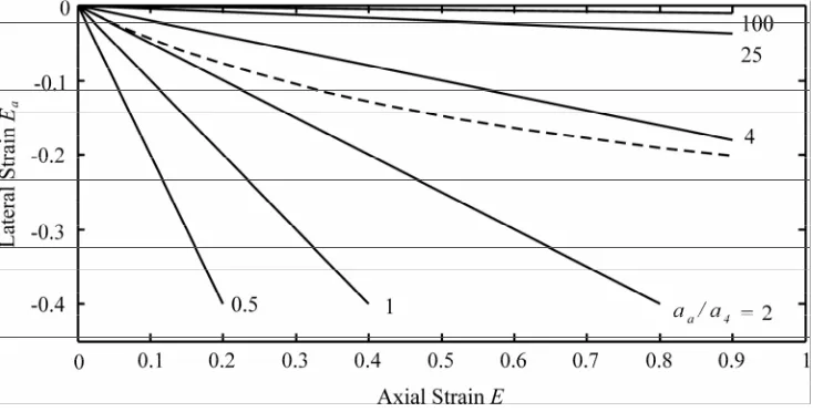
For several ratios a aa/ 4, a1, 2, Fig. 1 shows the dependence of lateral strain with
corresponding contraction is almost seven times larger, about 22.5 %), while for a aa/ 4 about
100 - the lateral contraction is below 1 %.
Fig. 1. Dependence of the lateral Green-Lagrange strain Ea, a = 1,2 on the strain in the loading
direction E during uniaxial tension for Fung’s two-dimensional exponential SEF (14). Isotropic path is represented by dashed line.
The tensional Piola-Kirchhoff stresses are
2 2
2
4 4
1 2 1 2
1 exp 1 , 1, 2
uni
a a a
a a
S ca E a E a
a a a a
(no sum on a) (18)
for tension in the directions 1 and 2. The condition uni 0 a
S leads to the convexity condition (16), i.e. if the values of material constants do not satisfy this condition there is no tensional stresses under simple uniaxial tension.
Material constants in (Fung et al. 1972) were determined by using the membrane assumption for inflation tests of artery specimens and 19 sets of material constants were obtained, which all satisfied the convexity condition (16). But, in 5 cases, for experiments denoted as 71:1, 71:2, 81:1, 81:2 and 81:3 one has a a1/ 425 so that the potential (14)
predicts an unrealistic contraction of specimen in direction 2.
In (Choung and Fung 1983) were evaluated 18 sets of material constants assuming 3D stress state for the same inflation experiments. Here, the SEF is not convex for 7 among these 18 cases (experiments denoted as 72, 72:1, 72:2, 81:2, 81:3, 82:2, 82:3) which means that Fung’s two-dimensional potential (14) predicts unrealistic stresses during uniaxial extension. In Table 1 are given values of ratio a aa/ 4, a1, 2 for the remaining 11 cases. Predicted contraction is not realistic (a a1/ 425) for 5 cases, for experiments denoted as 71, 71:1, 71:2,
78:1 and 81.
In (Takamizawa and Hayashi 1987) 16 sets of material constants were determined for Fung’s two-dimensional SEF (14) and material constant a4 is negative in 5 cases, which means
Exp. 71 71:1 71:2 78 78:1 78:2 78:3 81 81:1 82 82:1
a1/a4 37.6 105 95.3 9.1 68.1 10.7 13.1 25.2 5.9 9.1 4.4
a2/a4 53.3 107 48.6 0.9 32.0 1.0 1.5 32.4 0.7 4.4 0.7
Table 1. Values of ratios a1/a4 and a2/a4 for 11 material sets among 18 from (Choung and Fung
1983) for which Fung’s two-dimensional strain energy function (14) is convex.
3.2. Strain-Energy Function Proposed by Takamizawa and Hayashi
A two-dimensional SEF proposed in (Takamizawa and Hayashi 1987) has a logarithmic form
2 2
1 1 2 2 4 1 2
ˆ ˆ
ˆ Cln 1 Q , Q a E a E 2a E E
, (19)
where C0 is a stress-like material parameter; a a a1, 2, 4 are non-dimensional parameters, with the notation as for the above Fung’s model. The in-plane stresses for this model follow from (12):
1 1 1 4 2 2 4 1 2 2
1 1
2 ( ) ˆ, 2 ( ) ˆ.
1 1
S C a E a E S C a E a E
Q Q
(20)
This model was analyzed in (Humprey 1999) assuming constrained biaxial tension, with a conclusion that is not possible to find general conditions for material constants, as for Fung’s model, which provides positive stresses. However, the potential (19) is defined for 1 Qˆ 0
and from this condition follows that all material constants must be positive, just the same condition as for Fung’s model.
In the case of uniaxial loading, from the condition of zero lateral stress and expressions (20) follow the relations (17) for extensional paths. The uniaxial second Piola-Kirchhoff stress is
2 4
2 2
1 2 4
1 2 1
2 1 , 1, 2
1 1
uni
a a
a
a
S Ca E a
a a a
a E
a a
(no sum on a). (21)
In order to have positive uniaxial stress, the convexity condition (16) must be satisfied. Note that the strain energy function tends to infinity, as well as the stresses, when Qˆ1
(Holzapfel et al. 2000) which represents an additional restriction with respect to Fung’s model. Hence the model is only applicable for a limited range of states of deformation. Moreover, this strain energy function is convex under the same conditions (14).
Material constants for this model are given in (Takamizawa and Hayashi 1987), obtained from experiments on a dog carotid artery during inflation experiments, considering the artery as a thick-walled cylinder; and using two hypotheses: 1) the uniform strain hypothesis, and 2) the zero stress state in the reference configuration. By inspecting the constants it can be found that
4 0
3.3. Strain-Energy Function Proposed by Choi and Vito
Choi and Vito (Choi and Vito 1990) proposed a form of the exponential SEF (for canine pericardium) as
2 2
0 1 1 2 2 3 1 2
ˆ b exp(0.5b E ) exp(0.5b E ) exp(b E E ) 3
, (22)
where the constant b0 0 has the dimension of stress, while the other constants are
dimensionless; the axes and notation for the Green-Lagrange strains are as for the above models.
The main advantage of this model with respect to Fung’s model is that it is suitable for description of material behavior with very pronounced hardening characteristic. It has been applied to modeling of hyperelastic orthotropic membranes, as in either the case of abdominal aorta aneurism (Vande Geest et al. 2006), or natural and chemically treated pericardium (Choi and Vito 1990, Sacks and Choung 1998). We further demonstrate that this model can lead to an increase of lateral in-plane dimension under uniaxial loading.
The principal Piola-Kirchhoff in-plane stresses are now:
2
1 0 1 1 1 1 3 2 3 1 2
2
2 0 3 1 3 1 2 2 2 2 2
[ exp(0.5 ) exp( )],
[ exp( ) exp(0.5 )].
S b b E b E b E b E E
S b b E b E E b E b E
(23)
It was shown (Vande Geest et al. 2006) that all material constants must be positive in order to have positive stresses under constrained biaxial tension (strain behavior by Humprey).
In the case of uniaxial loading, the lateral in-plane Green-Lagrange strain cannot be expressed in an analytical form and it must be numerically determined from the condition either
2 0
S or S10 for a given strain E in the loading direction. If we denote the lateral in-plane strain by Ea (a2 for loading in direction 1, and a1 for loading in direction 2), then the zero lateral stress is expressed by the equation:
2
3 3
exp(0.5 ) exp( ) 0
a a a a a
b E b E b E b EE , a2,1 (no sum on a). (24)
Note that from this equation follows that the lateral strain is always less than zero, i.e. 0
a
E , since the coefficients b1, b2 and b3 and the strain E are positive.
The extreme value of Ea corresponds to the zero derivative, dE dEa/ 0, and from (24) it occurs when E 1/(b E3 a). Substituting this value into (24) and introducing a variable
2
0.5 a a
z b E , we obtain the equation
ln(2 )z z 1 0 (25)
which yields the solution z0.157185, and then
2 1 3 1 0.31437 cr b E b
, 1
2 3 1 0.31437 cr b E b
(26)
where 1
cr
E and 2
cr
Dog # #01 #04 #06 #08 #09
E1cr 0.51 0.15 0.23 0.44 0.40
E2cr 0.51 0.08 0.12 0.40 0.30
Table 2. Critical strains, calculated from (26), for uniaxial loading of dog canine pericardium. Model is defined by the two-dimensional exponential SEF (22) and constants obtained by
fitting biaxial experiments (Choi and Vito 1990)
We further analyze in detail whether the sets of material constants, obtained by fitting results of biaxial experiments, give physically realistic response of material when subjected to uniaxial loading. In Table 2 are given critical uniaxial strains E1cr and
2
cr
E calculated from material constants obtained by 5 experiments on dog canine pericardium (Choi HS and Vito RP, 1990). It can be seen that E1cr and E2cr are in the range of the strains reached in standard biaxial
tests (strains in experiments were up to 0.5). Therefore, using these constants, the model specified by the SEF (22) will give the lateral strain which is increasing when the uniaxial strain is above the critical values (26). This lateral strain increase cannot physically be justified.
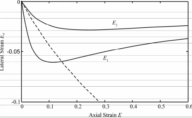
Fig. 2. Lateral stretch in terms of the stretch in the loading direction. Exponential SEF (22) proposed in (Choi and Vito 1990) and material constants for dog #06. The doted curve
corresponds to the isotropic case.
Figure 2 shows the dependence of lateral strain (eitherE2 or E1) in terms of the uniaxial
strain E, for loading in directions 1 and 2, and for the specimen #06 of Table 2. It can be seen that when loading is in direction 1, we have that the lateral strain E2 decreases, reaches
minimum at EE1cr 0.23, and then increases. On the other hand, for loading in the direction
the isotropic curve is also shown in the figure. The sets of material constants of other experiments lead to the results similar to these for the specimen #06.
We also give comments on material constants of the SEF (22) given in (Vande Geest et al. 2006), which are obtained by biaxial tests of squared specimen of Human Abdominal Aortic Aneurism (AAA). The 26 sets of material constants were inspected and we found that the critical strain for uniaxial loading lies in the range of the strains achieved in biaxial experiments for all sets of material constants, except for the specimen number 3.
3.4. Polynomial Strain-Energy Function Proposed by Vaishnav et al.
Vaishnav et al. (Vaishnav et al. 1972) proposed a 2D the strain energy function in a polynomial form for modeling the canine thoracic aorta:
2 2 3 2 2 3
1 1 2 1 2 3 2 4 1 5 1 2 6 1 2 7 2
ˆ c E c E E c E c E c E E c E E c E
, (27)
where the material constants ci, i1, 2,...7 have the dimension of stress. The Piola-Kirchhoff stresses follow from (12)
2 2
1 1 1 2 2 4 1 5 1 2 6 2
2 2
2 2 1 3 2 5 1 6 1 2 7 2
2 3 2 ,
2 2 3 .
S c E c E c E c E E c E
S c E c E c E c E E c E
(28)
Under constrained biaxial stretching, the stresses are:
2 2
1 2 1 1 3 4 1 , 2 2 1 5 1 ,
S c E c E S c E c E (29)
2 2
1 2 2 6 2 , 2 2 3 2 37 2 .
S c E c E S c E c E (30)
By analysis of the above relations it can be seen that all material constants must be positive for this case of biaxial loading in order to have tensional stresses. However, none of the sets of material constants given in (Vaishnav et al. 1972) and (Fung et al. 1979) satisfy these conditions, although the model (27) (for the fitted constants) show the material behavior prediction which agrees with the inflation experiments.
We illustrate our findings in Fig. 3. The constants used here are from Experiment 71 in (Fung et al. 1979), and are given in (kPa): c1 24.385, c2 3.589, c3 1.982,
4 46.334
c , c532.321, c63.743, c73.266. It can be seen that the stresses are negative
at the start of loading, Fig. 3a; and that the stresses are negative and small when straining is in the direction 2 (axial direction), Fig. 3b.
Fig. 3. Piola-Kirchhoff stresses in constrained biaxial loading, Experiment 71 in (Fung et al. 1979), polynomial SEF proposed in (Vaishnav et al. 1972). a) Loading in direction 1 (circumferential) and restrained deformation in axial direction; b) Loading in direction 2 and
restrained deformation in direction 1. (Strain behavior by Humprey).
4. Three-Dimensional models
Here, we consider 3D models with the strain energy function expressed in terms of the three principal Green-Lagrange strains, or in terms of the invariants specified below. Among these models, we analyze two-phenomenological Fung’s exponential model (Choung and Fung 1983), and the structural exponential model for artery layers (Holzapfel et al. 2000). As in Section 3, we investigated if the considered three-dimensional models predict physically realistic material response under the simple tension and constrained biaxial tension.
4.1. Strain-Energy Function of Fung’s type
A generalization of the model (14) to a three-dimensional regime (Choung and Fung 1983) assumes that the principal directions of the stress tensor coincide with circumferential, axial and radial directions of the artery (Holzapfel et al. 2000), labeled as the axes 1, 2 and 3, respectively. The strain energy function is given by
2 2 2
1 1 2 2 3 3 4 1 2 5 3 2 6 3 1
exp( ) 1 2
2 2 2
c Q
Q b E b E b E b E E b E E b E E
(31)
where c is stress-like material parameter and bi, i1,...6 are non-dimensional material parameters.
2 2
1 1 1 4 2 6 3 3 1 6 1 5 2 3 3
2 2
2 4 1 2 2 5 3 3 2 6 1 5 2 3 3
( ) ( ) exp( ),
( ) ( ) exp( ),
S c b E b E b E b E b E b E Q
S c b E b E b E b E b E b E Q
(32)
where the stretch 1 3 ( 1 2)
follow from the incompressibility condition (10).
In the case of uniaxial loading, the condition that the in-plane lateral stress is equal to zero can be expressed by the equation
4 3
4 3 1 0 0
p y p y p y p (33)
where 2
a
y is the squared stretch in the lateral direction. The coefficient p0 is
4
0 3
p b (34)
while pk, 1, 2,3k for uniaxial loading in direction 1 are
2 2
1 ( 3 5 6) 6, 3 4( 1) 2 5, 4 2,
p b b b b p b b b p b (35)
and for uniaxial loading in direction 2, the coefficients are
2 2
1 ( 3 5 6) 5, 3 4( 1) 1 6, 4 1.
p b b b b p b b b p b (36)
It is in general possible that, for a certain set of material constants, there can be a case when the solutions of equation (33) are not real, or that the real solution is out of the acceptable range of stretch (0,1), or that the lateral stretch is increasing during uniaxial tension.
We do not show here a graphical interpretation of biaxial or uniaxial loading, but summarize the results of the analysis of constrained biaxial and simple uniaxial tests. We have found that among 18 material sets, in 7 cases the stresses are negative under uniaxial loading (protocols: 72, 72:1, 72:2, 78:1, 82, 82:1, 82:3) and for 1 case in the constrained biaxial loading (protocol 82:2). Also stresses are close to zero in 3 cases for constrained biaxial loading (protocols 71:2, 72:1, 82:1).
4.2. Structural Strain Energy Function for the Artery Layers (Holzapfel et al, 2000)
The SEF introduced in (Holzapfel et al. 2000) describes a constitutive model which incorporates some histological structure of arterial walls (i.e. includes fiber directions) and consider each layer of the artery as a fiber-reinforced composite.
The basic idea of this model consists in the additive split of into a part iso, associated with isotropic deformations, and a part aniso associated with anisotropic deformations. Hence, the potential is written as
iso aniso
. (37)
The neo-Hookean model was used to determine the isotropic response of non-collagenous matrix material, so that iso is given as
1 1
( ) ( 3)
2
iso
c
I I
(38)
collagen fibers which represents the part aniso, the following expression was used in (Holzapfel et al. 2000):
2 1
4 6 2
4,6 2
( , ) {exp[ ( 1) ] 1}
2
aniso a
k
I I k I
k
(39)where I4 and I6 are the pseudo-invariants (Holzapfel 2007); k10 is a stress-like material
parameter, and k2 0 is a dimensionless material parameter. The anisotropic term aniso contributes only when the fibers are extended, i.e. when either I41 or I61, or both. The
above form of the SEF is used for two layers of an artery, i.e. for media and adventitia, with different sets of material constants.
According to the authors, “an appropriate choice of k1 and k2 enables the
histologically-based assumption that the collagen fibers do not influence the mechanical response of the artery in the low pressure domain to be modeled”. On the other hand, we will further show that under physiological domain of strains, when stretches 1, 21, the fibers are always stretched; while in the case of simple planar uniaxial tension, the value of stretch when the collagen fibers are activated, depends only on the angle of the fibers with respect to circumferential direction of the artery.
For a general biaxial deformation on a thin planar specimen excised from the arterial wall, which yields a plane state of stress, we have
2 2 2 2
4 6 1 cos 2 sin
I I . (40)
Since the model is symmetric with respect to interchange of I4 and I6 and principal axes
of stresses and deformations coincide (Ogden 2003), the principal Piola-Kirchhoff stresses for the model (37) follows from (13), by using 2
a a a
S :
4 2 2 2
1 1 2 1 4 2 4
2 4 2 2
2 1 2 1 4 2 4
(1 ) 4 cos ( 1) exp[ ( 1) ]
(1 ) 4 sin ( 1) exp[ ( 1) ]
S c k I k I
S c k I k I
(41)
where the anisotropic terms only contribute when the fibers are extended, i.e. when I4I61. General relations for the stresses in case of hyperelastic matrix reinforced by two families of fibers are given in (Ogden 2003).
Analyzing the expressions for stresses (40) in the case of simple planar uniaxial tension, we can reach the following conclusions. When the fibers are stretched, the anisotropic part of stress is positive, and in order to have zero lateral stress, the isotropic part of the lateral stress must be negative. This is possible only if the following condition between lateral stretch a and the stretch in the loading direction is fulfilled:
1/ 2
a
(42)
where a2 and a1 for loading in directions 1 and 2, respectively. This result agrees well with experimental findings in (Holzapfel 2006).
first 1 and 1/ 2 2
into equation (40) we obtain the stretch
1
aniso
, at the point at which
4 6 1
I I , as follows:
2
1
1 1 4 tan 1
2
aniso
. (43)
For the uniaxial extension in direction 2, it will be 2, 1 1/ 2. From that and
relation (40) we obtain the stretch 2aniso at the point at which is I4 I61,
2
2
1 1 4 / tan 1
2
aniso
. (44)
Therefore, the values of stretches in direction of uniaxial loading at which a fiber begins to extend, 1aniso and 2aniso, depend on the angle only, but not on the material constants.
Graphical representation of functions 1aniso( ) and
2 ( )
aniso
is shown in Fig. 4.
Fig. 4. Stretch at which the extension of fibers starts during simple planar uniaxial tension, in terms of the fiber angle . The structural SEF is introduced in (Holzapfel et al. 2000)
It can be seen that at uniaxial loading in the direction 1 and for (0, 54.7 )0 stretch of
fibers increases from the start of loading because 1aniso( ) 1 , while for 54.70 the
isotropic response occurs first, and the anisotropic response starts at stretch determined by equation (43). On the other hand, at uniaxial loading in direction 2, stretch of fibers starts from the beginning of loading for (35.3 , 90 )0 0 , while for 35.30 the deformation is first
Experimental extensional paths for adventitial layer of human aorta, consisting of nearly isotropic, transitional and anisotropic parts, are presented in (Holzapfel 2006). It has been shown here that the structural model for artery layers (Holzapfel et al. 2000) can predict the observed extensional paths for simple tension of tissue strip for limited range of fiber angles, i.e. for loading in direction 1 for 54.70 and for 35.30 when simple tension is in
direction 2.
Further, we note that for any biaxial straining when 1, 2 1, i.e. in physiological strain
domain which covers the cyclic inflation and axial extension of an artery (Holzapfel 2006), we have from (40) that I4 I61, with no dependence on the fiber angle ; hence, the fibers are
under stretch from the start of straining. This and the above uniaxial case represent the exceptions from the basic hypothesis in (Holzapfel et al. 2000) that by selecting the material constants k1 and k2 it is possible to interpret the (histologically-based) assumption that
collagen fibers do not affect the mechanical response of tissue in the low pressure domain. In the case of constrained biaxial loading when 2 1 and 1 , from (40) we obtain
2 2
4 1 ( 1) cos
I , and the stresses (41) are now
4 4 2 4 2 2
1 1 2
2 2 2 4 2 2
2 1 2
(1 ) 4 cos ( 1) exp[ cos ( 1) ],
(1 ) sin (2 ) ( 1) exp[ cos ( 1) ],
S c k k
S c k k
(45)
while for constrained biaxial loading when 11 and 2 we have I4 1 (21)sin2,
and the stresses (41) become
2 2 2 4 2 2
1 1 2
4 4 2 4 2 2
2 1 2
(1 ) sin (2 ) ( 1) exp[ sin ( 1) ],
(1 ) 4 sin ( 1) exp[ sin ( 1) ].
S c k k
S c k k
(46)
From relations (45) and (46) we see that isotropic parts of stress are not bigger than the material constant c, while the anisotropic part of stress is a function of cos4 in the first case
and of sin4 in the second case of loading. According to this, the anisotropic parts of stresses
for constrained biaxial tension are of the same order of magnitude only if fiber angle is close to 45 [o]. For example, for 2 and
2 1
k (common value in (Holzapfel et al. 2000) and (Holzapfel et al. 2004) is k21), and for 60 [o] or 30 [o], anisotropic part of stresses
is about 270 times larger in the case 1 than in case 2 of constrained biaxial loading. When
75
[o] or 15 [o], this ratio is about 34000. This leads to a conclusion that structural
model (37) – (39) might predict unrealistic ratio of anisotropy for constrained biaxial loading. Next, consider data given in (Holzapfel et al. 2004) where 18 sets of material constants for media and adventitia are determined using Fung’s 18 sets for the model (31) (Choung and Fung 1983). Five of these 18 sets for the model (37) – (39), experiments denoted as: 72, 78:1, 78:2, 82 and 82:2, for both media and adventitia have the constant c0, hence the uniaxial loading conditions cannot be modeled (see the above discussion about the finding that there must be a negative isotropic part of stress for proper modeling of uniaxial loading).
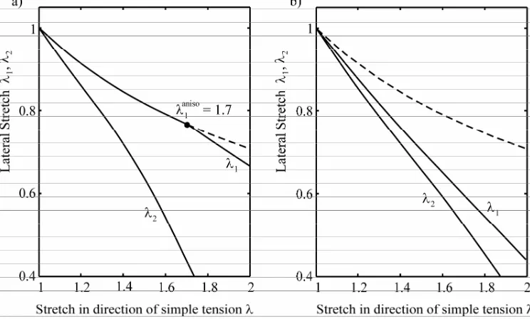
In Fig. 5 is shown the dependence of lateral stretch on the stretch in the loading direction, for simple uniaxial tension and material data for adventitia of a rabbit carotid artery (Holzapfel et al. 2004). Figure 5a corresponds to the experiment denoted as 71 (c0.7662 [kPa],
1 0.8255
k [kPa], k2 1.0301 and 65 [o]), while Fig. 5b is for experiment 71:2
(c0.9190 [kPa], k11.2061 [kPa], k2 1.2368 and 49[o]).
Fig. 5. Dependence of lateral stretches on the stretch in the loading direction (simple uniaxial tension), according to structural SEF introduced in (Holzapfel et al. 2000). Data for adventitia of a rabbit carotid artery (Holzapfel et al. 2004); a) Material parameters for experiment denoted
as 71 ( = 65o); b) Material parameters for experiment 71:2 ( = 49o). The dashed lines
represent the isotropic relationships.
The calculated strain paths are close to the experimental ones in (Holzapfel 2006) (not shown here) only when the loading is in direction 1 for experiment denoted as 71, where the isotropic response occurs first until the stretch is 1 1aniso1.7. As we discussed above, the
point at which straining of fibers starts during simple tension for structural model (37) – (39) is determined only by the value of fiber angle . On the other hand, the fibers are always stretched in the physiological strain domain for biaxial state of deformation, when 1, 21.
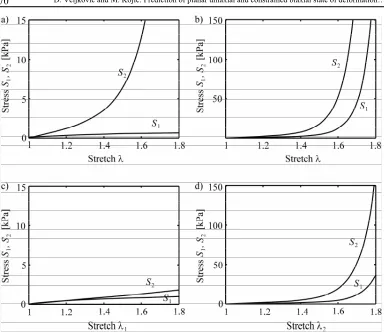
Fig. 6. Dependence of stresses according to structural SEF introduced in (Holzapfel et al. 2000). Material data for adventitia of a rabbit carotid artery for experiment denoted as 71 (Holzapfel et al. 2004); a) Simple uniaxial tension; b) Equibiaxial tension c) Constrained biaxial tension with
2 = 1; d) Constrained biaxial tension with1 = 1.
For the constrained biaxial loading, the isotropic part of stress (as mentioned above) is always lower then the value of material constant c. In this case, for experiment 71 in Holzapfel et al. (2004), value of c is c0.7662 [kPa], which means that isotropic part of stress is practically negligible. The fiber angle was found during fitting process in (Holzapfel et al. 2004) to be 65 [o]. Then, in the case of constrained biaxial tension in direction 1, when
2 1
, the anisotropic parts of stresses in (45) are about 100 times smaller than the stresses
(46) for the loading in direction 2. Obviously, this stress ratio is unrealistic.
By detailed inspection of the remaining 13 sets of material constant for media and adventitia given in (Holzapfel et al. 2004), we have found that there is no unrealistic prediction of stresses during simple tension and constrained biaxial tension only when the fitted value of fiber angle is close to 45 [o]. Note that in 6 cases for adventitia it was found 45 [o], which
5. Summary
A representative selection of two and three-dimensional anisotropic strain energy functions (SEFs) in common use in arterial mechanics has been investigated in this paper with respect to the mechanical response of tissue strips under planar uniaxial tension and constrained biaxial tension (strain behavior by Humprey). The goal of this simple study was to provide information which might be useful in a process of fitting material parameters for considered models, and in the evaluation of some alternative forms of strain energy function for arterial wall.
The two-dimensional SEFs were analyzed for the following models: exponential model (Fung et al. 1972), logarithmic model (Takamizawa and Hayashi 1987), exponential model (Choi and Vito 1990), and polynomial model (Vaishnav et al. 1972).
Convexity conditions for two-dimensional exponential Fung’s and logarithmic SEF were derived in (Holzapfel et al. 2000). Also, in (Humprey 1999) it was emphasized that all material constants must be positive in order to have tensional stresses under constrained biaxial tension. As we showed here, the convexity conditions for these models are equivalent to the conditions that a tensional stress develops and the lateral strain is decreasing under simple tension. Also, these SEFs predict unrealistic small or even negligible contraction in lateral direction during simple tension when the ratio of material constants a aa/ 4 a1, 2 is large. For example, when
4
/ 25
a
a a for a strain of 75 % in loading direction these two SEFs predict a contraction of only 3.5 % in lateral direction; while for a aa/ 4 about 100, the lateral contraction is below 1 %.
By inspection of material constants given in (Fung et al. 1979, Choung and Fung 1983, Takamizawa and Hayashi 1987), we found that in a significant number of cases the non-convex sets of material parameters were fitted because an unconstrained optimization was performed during the fitting processes. Hence, these two models cannot describe planar simple tension and/or constrained biaxial tension. Among the rest of material sets, there are cases when the prediction of lateral contraction under simple tension is unrealistic.
For the exponential model introduced in (Choi and Vito 1990), it is not possible to find an explicit expression for the extensional paths during simple tension, but this model always predicts unrealistic material response through the increase of lateral dimension. For the fitted material parameters from (Choi and Vito 1990), and (Vande Geest et al. 2006), we found that for all material sets the critical strains at which decreasing of lateral dimension starts is in the range of strains recorded in biaxial experiments.
Because of its cubic nature, the polynomial SEF with seven material parameters (Vaishnav et al. 1972) is not convex for any set of values of the material constants (Holzapfel et al. 2000). This character has a direct implication to adequate modeling of uniaxial loading. Since it is not possible to find the conditions for uniaxial loading in an analytical form we numerically investigated these conditions and found that all 27 sets of material constants in (Fung et al. 1979), and 3 sets in (Vaishnav et al. 1972) do not provide modeling uniaxial conditions. Also we found that all materials constants should to be positive in order to have tensional stresses during constrained biaxial tension according to (Humprey 1999).
The three-dimensional forms of the SEF considered here include: phenomenological exponential model (Choung and Fung 1983), and the so-called structural exponential model for the artery layers (Holzapfel et al. 2000).
acceptable range of stretches (0,1). Also, the lateral stretch can be non-monotonic or increasing during simple tension, or the predicted stresses are not tensional. We used material sets of (Choung and Fung 1983) to illustrate these unphysical predictions.
For the structural exponential model (Holzapfel et al. 2000), it was investigated the conditions when materials response turn from isotropic to anisotropic under uniaxial and biaxial tension. It was showed here that extension of tissue fibers in the isotropic hyperelastic matrix always occurs under biaxial loading when 1, 21. However, the point of the fibers activation under uniaxial tension depends on the angle of fibers only, rather than on material constants (Holzapfel et al. 2000). We showed that the structural model for artery layers can predict the extensional path in agreement with experiments in (Holzapfel 2006) for limited range of fiber angles only, i.e. for loading in direction 1 for 54.70 and for 35.30 when simple tension
is in direction 2. It is also showed that in the case of constrained biaxial tension, the anisotropic part of stress is the function of cos4 in case 1, and sin4 when loading is in direction 2.
Hence, when fiber angle is not close to 45o the model might predicts unrealistic magnitude of
stresses for constrained biaxial loading. For example, for experiment 71 in (Holzapfel et al. 2004) 65 [o], the anisotropic parts of stresses in the case of constrained biaxial tension in
direction 1 are about 100 times smaller than the stresses for the loading in direction 2, which might be unrealistic. By detailed inspection of material parameters from (Holzapfel et al. 2004), where 18 sets of material constants for media and adventitia were determined, we found that five of these sets for both media and adventitia have the constant c0, hence the uniaxial loading conditions cannot be modeled .
The presented analysis suggests that in experimental investigations, in order to establish a new computational model or to fit the constants for a selected model, uniaxial loading conditions should be considered together with constrained biaxial tension, in order to avoid inadequate model prediction of material response.
Acknowledgments
Извод
Предвиђање
раванског
једноосног
и
ограниченог
биаксијалног
стања
деформације
помоћу
уобичајено
коришћених
конститутивних
модела
у
механици
артерија
Dejan Veljković1, Miloš Kojić1,2,3
1 Bioengineering Research and Development Center, BioIRC, Sretenjskog ustava 27, 34000 Kragujevac, Serbia
2 Harvard School of Public Health,
665 Huntington Ave., Boston, MA 02115, U.S.A. [email protected]
3 Department of Nanomedicine and Biomedical Engineering, University of Texas Medical Center at Houston,
1825 Pressler Street,Houston, TX 77030, U.S.A.
Резиме
Уовомрадујеистраживанмеханички одзивисечакаткиваприраванскомједноосном и
ограниченом биаксијалном затезању (деформационо понашање према Хамфрију
(Humprey)) зарепрезентативниизбордво- итро-димензионалнефункциједеформационе енергије, уобичајенокоришћене умеханициартерија: Фангови (Fung) 2Ди 3Д модели,
логаритамски, полиномиалнииекспоненцијалниЧои иВито (Choi и Vito) 2Дмодели, и структурални експоненцијални 3Д модели за слојеве артерије. Показано је да сви ови модели имају ограничења у могућности описивања посматраних стања деформације.
Коришћењемпараметараизлитературеутврђеноједапостојизначајанбројслучајевагде се може предвидетинереални одзив материјала, акосу параметриван опсегаукоме је изведенпроцесфитовања. Дабисеизбегланестабилностизрачунатогодзиваматеријала,
сугерирамо да треба да се размотре једноосни услови оптерећења, заједно са ограниченимбиаксијалнимзатезањем, уексперименталнимистраживањимаприувођењу новогматеријалногмодела, илиприфитовањуконстантиизабраногмодела.
Кључне речи: биаксијално тестирање, артеријски зид, конститутивно моделирање,
коначнедеформације, функцијаенергиједеформације
References
Choi HS and Vito RP (1990). Two-dimensional Stress-Strain Relationship for Canine Pericardium, Journal of Biomechanical Engineering; 112(2): 153-159. DOI:10.1115/1.2891166.
Choung CJ and Fung YC (1983). Three-dimensional Stress Distribution in Arteries. Journal of Biomechanical Engineering; 105: 268-274.
Fung YC (1984). Biomechanics, Springer, New York.
Hildebrandt J, Fukaya H and Martin CJ (1969). Stress-strain relations of tissue sheets undergoing uniform two-dimensional stretch. Journal of Applied Physiology; 27(5): 758-762.
Holzapfel GA, Gasser CT and Ogden RW (2000). A new constitutive framework for arterial wall mechanics and comparative study of material models. Journal of Elasticity; 61(1-3): 1-48. DOI: 10.1023/A:1010835316564.
Holzapfel GA, Gasser CT and Ogden RW (2004). Comparison of a Multi-Layer Structural Model for Arterial Walls With a Fung-Type Model, and Issues of Material Stability.
Journal of Biomechanical Engineering; 126(2): 264-275. DOI: 10.1115/1.1695572
Holzapfel GA and Ogden RW (2008). On Planar Biaxial Tests for anisotropic Nonlinearly elastic solids. A Continuum Mechanical Framework. Mathematics and Mechanics of Solids; 14(5): 474-489. DOI:10.1177/1081286507084411.
Holzapfel GA (2006). Determination of material models for arterial walls from uniaxial extension tests and histological structure. Journal of Theoretical Biology; 238(2): 290–302. DOI: 10.1016/j.jtbi.2005.05.006
Holzapfel GA (2007). Nonlinear Solid Mechanics, John Wiley & Sons.
Humprey JD (1984). And Evaluation of Pseudoelastic Descriptors Used in Arterial Mechanics.
Journal of Biomechanical Engineering 1999; 121(2): 259-262. DOI:10.1115/1.2835113. Ogden RW (2003). Nonlinear Elasticity, Anisotropy, Material Stability and Residual Stresses in
soft Tissue. In Holzapfel GA and Ogden RW. eds., Biomechanics of Soft Tissue in Cardiovascular Systems. CISM Courses and lectures 441: 65-108. Springer-Verlag, Wien, New York.
Sacks MS and Choung CJ (1998). Orthotropic mechanical properties of chemically treated bovine pericardium. Annals of Biomedical Engineering; 26(5): 892-902. DOI:
10.1114/1.135
Takamizawa K and Hayashi K (1987). Strain energy density function and uniform strain hypothesis for arterial mechanics. Journal of Biomechanics; 20(1): 7-17.
Vaishnav NR, Young JT, Janicki JS and Patel DJ (1972). Nonlinear Anisotropic Elastic Properties of the Canine Aorta, Biophysical Journal; 12(8): 1008-1027.