Paper 06-2016-1

Some Aspects of Computation Methods in Strength Analysis of Flight

Structures

S. Maksimović1, I. Vasović2, K. Maksimović3

1 Military Technical Institute, 1 Ratka Resanović Street, Belgrade, Serbia

e-mail: [email protected]

2 _{Institute GOŠA, Belgrade}

e-mail: [email protected]

3 _{Republic Serbia, City Administration of City of Belgrade,}

Secretariat for Utilities and Housing Services Water Management, Kraljice Marije Street, Belgrade, Serbia

e-mail: [email protected]

Abstract

Primary attention of our investigation during the last ten years has been focused on the development of efficient computation methods and corresponding software for strength analyses of flight structures such as aircraft, helicopter and tactical UAV structures. In these investigations the complete computation methods/procedures are developed and corresponding in-house software for total fatigue life estimations (up to crack initiation and crack growth) of structural components under general load spectrum. In order to ensure efficient computation methods in fatigue life estimations of metal structural components the same low cycle fatigue material properties are used for initial fatigue life estimations and residual fatigue life estimations. The developed computation methods and corresponding software are verified using our own experiments. Most of these methods/procedures and software were applied for the extension of aircraft structure lifetime, both those at home and those in service abroad. An important aspect in designing and extending the life of the aircraft structure represents a precise determination of the load. For this purpose, as a rule, CFD numerical simulations are used. It is especially important to accurately determine the load of the main and tail rotor blades of the helicopter. In these cases, the application of CFD numerical simulation is unavoidable.

Keywords: Flight structures, Fatigue, Computation methods, CFD, Fatigue life estimation

1. Introduction

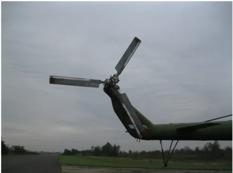
to use the properties of the materials as efficiently as possible. One way to improve the fatigue life predictions may be to use relations between crack growth rate and the stress intensity factor range. To determine residual life of damaged structural components two crack growth methods are used here: (1) conventional Forman`s crack growth method and (2) crack growth model based on the strain energy density method. The last method uses the low cycle fatigue properties in the crack growth model (Maksimovic 2012). In Figures 1 and 2 representative structure of helicopter and aircraft are shown in which presented computation procedures can be used. Figure 1 shows the composite helicopter tail rotor blades with metal fittings.

Fig. 1. The helicopter tail rotor

Fig. 2. Structure of aircraft Super Galeb G-4

2. Definition of load spectra for helicopter tail rotor blades using CFD method

Semi-empirical methods were being widely used in calculation of helicopter blade aerodynamic load, such as lifting line theory combined with airfoil experimental data, given as a function of the local angle of attack and Mach number. But, in such approach empirical corrections had to be included in order to take into consideration the effects of the dynamic stall, compressibility and blade interaction with trailing vortex. Today, powerful CFD methods are mostly used in helicopter aerodynamic load determination. In this way the empirical corrections are avoided.

In the paper, CFD software package ANSYS FLUENTsoftware code is used for obtaining aerodynamic load of the Mi-8 helicopter tail rotor blades. The tail rotor thrust primarily serves to balance the main rotor torque. However, due to wide diapason of the blade pitch change and large Coriolis forces caused by the blade flapping, the tail rotor blades work in much severe conditions compared to the main rotor blades. The tail rotor failure could cause serious accident and, because of that, reliable methods must be used in the calculation of aerodynamic load of the tail rotor blades.

Assuming that the tail rotor thrust moment balances the main rotor torque, thrust is calculated from

l

T

where M and lt are the main rotor torque and the distance of the tail rotor from the helicopter

center of gravity respectively. The corresponding thrust coefficient can be obtained from (Boljanovic еt al. 2016) as

( )

R

A

s

T

t

Ω

where air density, solidity, rotor area and tip speed of the tail rotor are denoted by ρ, st, At and

(ΩR)t respectively. In forward flight, the tail rotor axis is perpendicular to the flight direction,

i.e. the incidence of the no-feathering axis of the tail rotor is zero. Tail rotor flow regime is defined by advance ratio μt and inflow ratio λt respectively

R

V

Ω

=

α

µ

cos

λ

α

λ

R

V

−

=

Ω

sin

where αt is the incidence of the no-feathering axis of the tail rotor.

In forward flight, the only contribution to the inflow ratio λt is the induced velocity ratio λit,

i.e.

λ

λ

=

−

while

µ

λ

t

s

2

Now the required tail rotor collective-pitch angle to trim can be calculated from













₊











 +

=

λ

µ

θ

t

t

_a

t

4

2

3

1

2

3

if tct is given. The chord and pitch angle are constant along the tail rotor blade, i.e. the tail rotor

blades are without taper or twist. Thus each blade is rotated about its longitudinal axis through θot relative to plane perpendicular to the no-feathering axis.

In forward flight there is flow asymmetry for advancing and retreating blade. The different lift forces appear on the blades causing rolling moment about the helicopter longitudinal axis. This moment is compensated by a hinge that provides blade flapping toward the plane perpendicular to the no-feathering axis. The flapping angle is a periodic function of the azimuth angle and can be expressed by the Fourier series of the form

... 2 sin 2 cos sin

cos _{1 2 2}

1

0− − − − −

= ψ ψ ψ ψ

β

_a

_a

_b

_a

_b

Experiments show that coefficients beyond the second order are small quantities compared to the ones of the first order and can be neglected. For most steady regimes coefficients of the second order can also be omitted thus simplifying calculation considerably. As a rough rule, the value of a coefficient of some order is about one tenth of the previous lower one. The coefficients ao, a1 and b1 depend on the rotor flow regime, collective-pitch angle and Lock's

inertia number γ. Neglecting tail rotor flapping-hinge offset, the coefficients become









_

₋









 +

=

γ

θ

µ

λ

t t

a

1

₃

4

8

θ

λ

µ

µ

a

3 4

2 1

2 ₍₁₀₎

(

)

2 1 3 4 0 2

1

µ

λ

µ

t

a

b

while γ is defined as

G

R

ρ

γ

where a, c, Rt and Gt are lift slope of the tail rotor airfoil, tail rotor chord, radius and weight respectively.

However, blade flapping can be realized from different point of view. Namely, each blade traces out a cone, whereas the blade tips trace out the base of the cone which is often referred to as the tip-path plane, i.e. blades move steadily in the tip-path plane. The axis of the cone is no-flapping axis, tilted relative to the no-feathering axis. The cone with no-no-flapping axis is obtained rotating plane perpendicular to the no-feathering axis through the angles –b1 and a1

X axis is directed to the flight direction. The no-flapping axis cone is modeled in the numerical simulation.

The Coriolis force appears due to blade flapping, acting in the chord plane of each tail rotor blade segment. Its value can be obtained as

β

β



r

m

F

=

2

∆

Ω

where Δm and r are segment mass and distance from the axis of rotation. These forces are much larger than aerodynamic drag forces at each segment, giving moment about the rotor shaft which is balanced by the moment of centrifugal force. This happens through lagging motion if drag hinges exist. Mi-8 tail rotor blades have no drag hinges, so large alternating moments occur that mostly determine dynamic strength and fatigue life of the blade.

The following input data are used in calculating tail rotor loads: number of blades N=3, blade airfoil NACA 230M, rotor area At=11.4 m2, rotor diameter Rt=3.81 m, blade twist ε=0o,

rotor solidity σ=0.136, blade chord c=0.271 m, rotor rpm n=1124, blade mass m=13.5 kg, distance from helicopter c.g. to tail rotor axis lt= 12.646 m, helicopter forward speed V=56.25

m/s, advanced ratio μt= 0.251, induced velocity ratio λit= 0.0196.

The results are given for forward flight at speed equal to 0.9 VNE (never exceeded).

According to representative statistical data (Fielding, J.P. 1999), transport spectrum flight at this speed lasts almost 30% of the total flight time.

Having determined tail rotor thrust, its flow regime, collective-pitch angle and coefficients of the Fourier series that describe the flapping angle as a function of the azimuth angle, numerical simulation was accomplished using the CFD software in order to obtain distributions of aerodynamic forces along each blade span. The Navier-Stokes equations are solved in the software. This equation in the so-called conservation form (Brislow 1985) can be written as

B

t

U

x

G

x

F

=

∂

∂

+

∂

∂

+

∂

∂

where U, Fi, Gi and B are the conservation flow variables, convective flux variables, diffusion flux variables and source terms, respectively





















=

E

U

_v

ρ

ρ

ρ

























+

+

=

v

v

v

v

v

F

p

E

p

i

ρ

ρ

ρ

δ

























+

−

−

=

q

v

G

τ

τ

0

























=

v

F

F

B

ρ

ρ

0

i,j = 1,2,3,

with ρ, vj, Fi, E, p, τij, qi being density per unit mass, components of the velocity vector, components of body force vectors, total energy, pressure, viscous stress tensor and heat flux respectively. Kronecker delta is denoted with δij where δij = 1 for i=j and δij = 0 for i≠j. The total energy given as a sum of the internal energy per unit mass e and kinetic energy

v

v

e

E

2

1

+

=

(

)











 −

−

=

_v

_v

j j

E

p

2

1

1

ρ

γ











 −

=

_v

_v

c

v

E

T

2

1

1

with cv being the specific heat at constant volume. Integrating equation (14) spatially over the

volume of the domain,

∫

=

Ω

















−

∂

∂

+

∂

∂

+

∂

∂

0

d

B

t

U

x

G

x

F

another form of the governing equations can be obtained as

(

+

)

Γ

=

0

+

Ω













₋

∂

∂

∫

∫

d

d

B

t

U

n

G

F

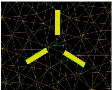
The surface integral in equation (19) represents the convection and diffusion fluxes through the control surfaces. The integral form enables appropriate resolving for discontinuous flows with shock waves because conservation properties across the discrete element boundary surfaces are satisfied. This approach is the basis for the finite volume method applied in the used software. There are two steps in the numerical simulation. In the first step, the mesh is generated in the domain, while in the next step, flow field is determined around the tail rotor blades. The volume mesh is composed of 1 327 763 cells and one part of this mesh is shown in Figure 3.

Fig. 3. Volume mesh around the tail rotor blades

Fig. 4. Gauge static pressure on the upper sides of the blades

The blades rotate counterclockwise. The zone of the lowest pressure appears on the advancing blade, immediately behind the leading edge and near the blade tip. The pressure distribution on two retracting blades is rather similar, because the flow conditions at these two positions are similar.

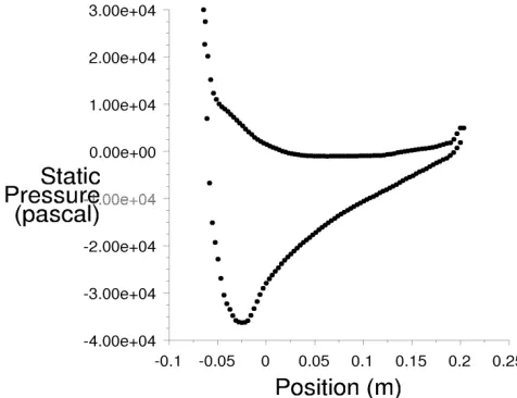
Gauge static pressure distribution along the chord of the advancing blade at 75% of the blade span can be seen in Figure 5.

Fig. 5. Gauge static pressure distribution along the chord of the advancing blade at 75% of the span

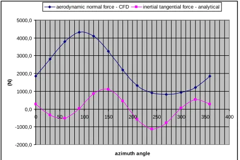
Fig. 6. Relative Mach number around airfoil at 75 % of span of the advancing blade The aerodynamic force normal to blade chord plane and inertial force in the chord plane, acting on the blade during one revolution, are shown in Figure 7. It can be seen that magnitudes of the

Fig. 7. Aerodynamic normal force and inertial tangential force change during one revolution inertial and aerodynamic normal force are of the same order. Large alternating moments at the tail rotor hub are caused by the inertial force. Together with two oscillations per revolution, these moments dominantly influence blade dynamic strength and fatigue life.

3. Initial fatigue life estimation of structural components

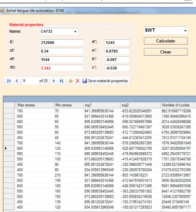
Computation procedure for fatigue life estimation of representative structural element (Fig. 8) and real metal structural element of helicopter tail rotor blade (Fig. 9) are presented here. To define the computation procedure, one component with a hole under cyclic load is considered. For this purpose, Smith-Watson-Topper (SWT) curve is used to determine the number of cycles up to initial damage:

-2000,0 -1000,0 0,0 1000,0 2000,0 3000,0 4000,0 5000,0

0 50 100 150 200 250 300 350 400

azimuth angle

(N)

( )

( )

( )

SWT E N E N

2

P = σ ∆ε = σ + σε + (20)

2

m max

σ ∆ + σ = σ

where: K', σf’, εf', b, c are low cyclic material properties, sm - the mean stress, smax- the

maximum stress, Nf- number of cycles to initial damage. Neuber`s rule is usually used to

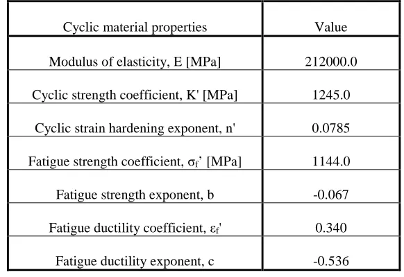
calculate elastic-plastic stress and strain at the roots or notches from their entirely elastic theoretical equivalents that might be estimated by an elastic FE analysis. Low cyclic fatigue properties of steel 4732 are determined experimentally (Table 1) using servo-hydraulic MTS test system.

Cyclic material properties Value

Modulus of elasticity, E [MPa] 212000.0

Cyclic strength coefficient, K' [MPa] 1245.0

Cyclic strain hardening exponent, n' 0.0785

Fatigue strength coefficient, σf’ [MPa] 1144.0

Fatigue strength exponent, b -0.067

Fatigue ductility coefficient, εf' 0.340

Fatigue ductility exponent, c -0.536

Table 1. Low cyclic fatigue properties of steel 4732

Fig. 8. Representative structural element (plate with hole, material C 4732) (kt=3.342; W=

60mm, t= 5 mm d= 17.5mm)

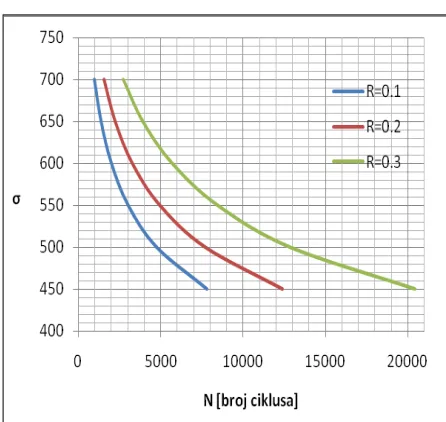
Detail computation initial fatigue life of structural element, Fig.8, for different stress levels and stress ratios R are given in Table 2 and Fig. 10.

Fig. 9. Real structural element of helicopter tail rotor blade made from material C 4732

X Y

Z

240.5

226.1

211.7

197.3

182.9

168.5

154.1

139.7

125.3

110.9

96.5

82.1 67.7

53.3

38.9

24.5 10.11

V1 L1 C1

Table 2. Initial fatigue life estimation of structural components (plate with hole, Fig. 8) Results presented in Table 2, for representative structural element (plate with hole), and different load levels using low cyclic material properties can be used for initial fatigue life estimations(Maksimović 2005; Boljanovic еt al. 2016) of every complex structural element. For precise determination of stresses in structural components, MSC/NASTRAN software code is used.

4. Conclusions

aerodynamic load distributions, CFD analysis is used. Elastic-plastic FE stress analysis around notches with SWT criteria is developed as a procedure for initial fatigue life estimation of metal structural components to helicopter tail rotor blades. Combining CFD analysis for aerodynamic load computations with computation procedure for initial life estimation achieves real conditions for reliability design of metal structural components of helicopter tail rotor blades. In practical extension life of an aircraft structure such as aircraft Super Galeb G-4 combined NDT and initial fatigue life estimation methods are used. For this purpose in-house software is used for initial fatigue life estimations of complex aircraft structural components.

Acknowledgments This work was financially supported by the Ministry of Education, Science and Technological Development of Serbia under Projects TR-35011 and TR-35045.

Извод

Кратак осврт на рачунске методе коришћене у анализи чврстоће

структура летелица

С. Максимовић1, И. Васовић2, К. Максимовић3

1 Војно_-технички институт, Ратка Ресановића 1, Београд, Србија

имејл: [email protected]

2 Институт ГОША, Београд

имејл: [email protected]

3 Градска управа града Београда, Секретеријат за комуналне и стамбене послове,

Краљице Марије 1,Београд Србија имејл: [email protected]

Резиме

Кључне речи: летелице, замор, рачунске методе, ЦФД, процена заморног века

References

Boljanovic S., Maksimovic S., Djuric M. (2016). Fatigue strength assessment of initial semi-elliptical cracks located at a hole, International Journal of Fatigue, Volume 92, Part 2,

pages 548–556.

Brislow, J.W. (1985) Structural Integrity of Helicopters in Relation to their Airworthness, The Int. Journal of Aviation Safety.

Chung, T.J. (2002). Computational Fluid Dynamic. Cambridge University Press.

Edwards, K. L and Davenport, C. (2006). Materials for rotationally components: rationale for

higher performance rotor-blade design, Materials and Design, 27, 31-35.

Fielding, J.P. (1999). Introduction to aircraft design. Cambridge University Press.

Maksimović K., Đurić M., Janković M. (2011). Fatigue Life Estimation of Damaged Structural Components Under Load Spectrum, Scientific Technical Review, Vol. 61, No.2, pp.16-23. Maksimovic S., Kozic M., Stetic-Kozic S., Maksimovic K., Vasovic I. (2014). Maksimovic M.,

Determination of Load Distributions on Main Helicopter Rotor Blades and Strength Analysis of the Structural Components, Journal of Aerospace Engineering, Vol. 27, Number 6, November/December 2014.

Maksimović S., Vasović I., Maksimović M., Đurić M. (2013), Improved computation method to fatigue and fracture mechanics analysis of aircraft structures, Fourth Serbian (29th Yu) Congress on Theoretical and Applied Mechanics Vrnjačka Banja, Serbia, 4-7 June 2013, pp 335-340.

Maksimović, S. (2005). Fatigue life analysis of aircraft structural components. Scientific

Technical Review, vol. LV, No. 1, p. 15-22.

Maksimovic, S. (2012) Computation methods in residual fatigue life estimations of structural

components using strain energy density method, Journal of the Serbian Society for

Computational Mechanics / Vol. 6 / No. 1, pp. 74-82 ANSYS FLUENT software code