http://www.sciencepublishinggroup.com/j/earth doi: 10.11648/j.earth.20190803.16
ISSN: 2328-5974 (Print); ISSN: 2328-5982 (Online)
A Weighting Inversion Method of Spectrum Induced
Polarization
Wu Yu Hao
1, 21
Tianjin Institute of Geotechnical Investigation and Surveying, Tianjin, China
2College of Geo-exploration Sciences and Technology, Jilin University, Changchun, China
Email address:
To cite this article:
Wu Yu Hao. A Weighting Inversion Method of Spectrum Induced Polarization. Vol. 8, No. 3, 2019, pp. 178-189. doi: 10.11648/j.earth.20190803.16
Received: December 28, 2018; Accepted: May 23, 2019; Published: July 4, 2019
Abstract:
The inversion results of complex resistivity method are four Cole-Cole model parameters. Among the four parameters, the frequency dependence and the time constant are more difficult to invert. It is necessary to study an algorithm that can invert the four Cole-Cole model parameters at the same time. In this paper, the least squares and OCCAM inversion algorithms are used to invert four Cole-Cole model parameters. In other words, two model constraints are added to the objective function. When inverting different Cole-Cole model parameters, the real and imaginary parts of the data are weighted to adjust the proportion of real part and imaginary part of data in inversion. Firstly, the formula of the algorithm is deduced. Then the theoretical models are designed for inversion trial calculation. In the inversion process, the inversion converges steadily by adjusting the Lagrange factor, and the inversion effect is improved by adjusting the weighting coefficients of real part and imaginary part. This method can get better inversion results by adjusting the proportion of the real and imaginary parts of the data in the inversion. The model trial results show that the weighting inversion algorithm significantly improves the results of the inversion of the four Cole-Cole parameters.Keywords:
Spectral Induced Polarization, Cole–Cole Model Parameters, Occam Inversion, The Least Squares Inversion, Weighting Inversion1. Introduction
Spectrum induced polarization (SIP), also known as complex resistivity method (CR), is widely used in environmental and engineering, mineral and land pollution exploration, and based on the difference of electrochemical properties between rocks and ores. The characteristic of this method lies in the abundant parameters used for interpretation. Pelton [11] published a famous paper "Removal of electromagnetic coupling and recognition of ore-bearing anomalies in multi-frequency IP". Cole-Cole model is introduced into geophysics. Cole-Cole model and its combination are used to fit the induced polarization and electromagnetic coupling, thus laying the foundation of SIP, and he thought that the frequency dependence c and the time constant τ could be used to distinguish mineral from non-mineral. put forward the theory that the approximate formula is used as the forward model to obtain the true parameters of SIP from a measuring point. Liu Song et al. [6]
invert the other three Cole-Cole model parameters by using phase. On the basis of neglecting the electromagnetic coupling effect, Zhou Feng [15] improves the algorithm of Ghorbani et al. [1]. In complex resistivity inversion, he regards the resistivity model obtained by DC inversion as the initial model of zero-frequency resistivity. After that he no longer updated the zero-frequency resistivity parameter and invert chargeability m, the frequency dependence c and the time constant τ by using phase of complex resistivity. Fan Cuisong [3] proposed a joint inversion algorithm of electric field amplitude and phase, and simultaneously inverted four Cole-Cole parameters.
Because the real part and imaginary part of complex resistivity are different in sensitivity to different Cole-Cole parameters, and the order of magnitude of the real part is generally much larger than that of the imaginary part. This often results in that the degree of imaginary part fitting is still very low when the fitting error has reached the preset threshold value, and it cannot obtain the desired results of the frequency dependence c and the time constant τ which have a greater impact on the imaginary part of complex resistivity. In order to solve this problem, based on the consideration of electromagnetic coupling, a weighting inversion algorithm using the real and imaginary parts of complex resistivity is proposed. It is adopted that inverting zero-frequency resistivity ρ0 and chargeability m firstly, then inverting the frequency dependence c and the time constant τ. The inversion algorithm is deduced, and then test several theoretical models show on the stability and superiority.
2. D Weighting Inversion of Real and
Imaginary Parts of SIP Data
2.1. Damped Least Squares Inversion Theory
When calculating the inversion problem of complex resistivity, we set it on a field electrical layout with N observation data di, defined mi as one of Cole-Cole parameters, i=1,2,···M, defined M as the number of layers of underground model, defined F(m) as the forward data, and defined Wd as the covariance matrix of observation data. Its structure is as follows:
d 1 i N σ σ σ = W ⋱ ⋱ (1)
According to Shang Tongxiao [13], the objective function Φ is defined as follows:
(
)
T(
)
d d
Φ=W d F(m)− W d F(m)− (2)
Define model constraints as follows:
( ) ( )
T mΦ =α ∆m ∆m (3) In the formula, α is the damped factor.
This paper modifyed the objective function to:
d m
Φ=Φ +Φ (4) Taylor's expansion of forward data F(m) is as follows:
k k
F(m +∆m)=F(m )+ ⋅J ∆m (5) In the formula, mk is the initial model of the first iteration, J is the Jacobian matrix, whose element is ij i k
j
F (m ) J
m
= , ∆m
is the modification of the model.
By introducing formula (5) into formula (4), the linearized objective function is obtained:
( )T ( ) ( ) ( )T
d d
Φ=W d−F(m)− ⋅J ∆m W d−F(m)− ⋅J ∆m +α ∆m ∆m (6) From the above formula, we can see that the function Φ is function of variables ∆m, and we take the extreme condition for the objective function, as follows:
0 ∆m ∂ = ∂ Φ (7)
It is simplified and gained the damped least squares linear inversion equation:
(
) (
T)
1(
)
(
( )
)
d d d k
∆m=W J W J +αI− W J d−F m (8)
Given the initial model mk, the model modification ∆m
can be obtained from the formula (8), and the next iteration
k 1 k ∆
m + =m + m as a new initial model can be obtained until the fitting difference is less than the pre-given threshold value,
k 1
m + is the final inversion result.
2.2. 1D Weighting Inversion of Real and Imaginary Parts of SIP Data
different weighting coefficients are taken. The inversion objective function is established as follows:
1 Re 2 Im
Φ= ⋅λ Φ +λ ⋅Φ
(9)
In the formula, ΦRe and ΦIm respectively represent the objective functions of the real part and the imaginary part of complex resistivity, λ1 an dλ2 are weighting coefficients. Among them, ΦReandΦIm is as follows particularly:
(
)
(
)
(
)
(
)
T
Re Re
Re d Re Re d Re Re T
Im Im
Im d Im Im d Im Im
Φ Φ = − − = − −
W d F (m) W d F (m)
W d F (m) W d F (m)
(10)
In the formula, dRe and dIm respectively are the real part and the imaginary part of the observation data, FRe
( )
m and( )
Im
F m respectively are the real part and the imaginary part of the forward data, WdRe and
Im d
W respectively are the covariance matrix of the real part and the imaginary part of the observation data.
According to the theory of the previous chapter, model constraints Φm =α
( ) ( )
∆m T ∆m are added to the objective function and the formula (2.9) is rewritten as follows:Re Im m
Φ= ⋅λ1 Φ + ⋅λ2 Φ +Φ
(11)
Referring to the deduction process of the damped least squares inversion mentioned above, the (11) formula is linearized and approximated, and then under the premise of
0 m ∂Φ =
∂∆ , the linear equations of the weighting inversion are
obtained, as follows:
(
) (
)
(
)
(
( )
)
(
) (
)
(
)
(
( )
)
1 T
Re Re Re
1 d Re d Re d Re Re Re k
1 T
Im Im Im
2 d Im d Im d Im Im Im k
∆ λ α
λ α
m W J W J I W J d F m
W J W J I W J d F m
− − = + − + + − (12)
In the formula, JRe and JIm which are the Jacobian matrices of the real part and the imaginary part of the SIP data respectively, will be obtained by method of difference.
The fitting difference of each iteration of inversion
is defined as:
*
Re Im
Φ =Φ +Φ
(13)
3. Inversion Results and Analysis
3.1. Damped Least Squares Inversion Results and Analysis
In this section, we will test the effectiveness and superiority of the weighting inversion algorithm by calculating several theoretical models. In the following two examples, the observation SIP data are both real and imaginary parts of observation complex resistivity, and the dipole-dipole measuring device is adopted. The number of array is 1, each array has 30 measuring points, and the length from transmitting to receiving dipole is 100m. There are seven observation frequencies, respectively: 0.0001Hz, 0.001Hz, 0.01Hz, 0.1Hz, 1Hz, 5Hz, 10Hz.
This paper uses two-step inversion method that the inversion consists of two steps: the first step is to invert the zero-frequency resistivity and chargeability without changing the values of the fixed time constant and frequency dependence. The second step is to invert the frequency dependence and time constant by taking the inversion results of the first step as the initial model and without changing the values of the zero-frequency resistivity and chargeability. Table 1. Polarization model of two layers.
parameters Zero-frequency resistivity chargeability time constant frequency dependence Layer thickness
ρ1 ρ2 m1 m2 τ1 τ2 c1 c2 h1 h2
true value 50 300 0.3 0.7 5 15 0.15 0.3 300 +∞
Initial 1 10 10 0.45 0.45 10 10 0.2 0.2 300 +∞
Initial 2 10 10 0.45 0.45 15 5 0.3 0.15 300 +∞
Initial 3 10 10 0.45 0.45 8 8 0.18 0.18 300 +∞
Initial 4 10 10 0.45 0.45 2 5 0.35 0.25 300 +∞
Fitting deference of initial 1 0.0247
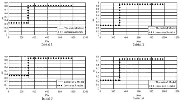
(Fitting difference is one after inversion of the second step) Figure 1 to Figure 2 show the inversion results of zero-frequency resistivity ρ0and chargeabilitymwhen the initial values of frequency dependence c and time constant
τ
are different. When the weighting coefficients are taken as follows: λ1=100000,2 =1
λ , fixed frequency dependence
and time constant are unchanged, and only zero-frequency resistivity ρ0 and chargeability m are inverted.
Table 1 shows that the initial values of zero-frequency resistivity ρ0 and chargeability mare the same in initial
The inversion examples calculated above are all carried out under the condition that the difference between the initial value and the true value of each parameter is not large in a certain range. When the difference between the initial value and the true value of the model is too large, the inversion often falls into the local minimum, which is caused by the defect of the damping least square method itself. Based on the above analysis, we uses two-step inversion method to calculate the following inversion examples, that is, first to invert zero-frequency resistivity ρ0 and chargeability m, second to invert frequency dependence c and time constant
τ
.The first step: the values of fixed frequency dependence c and time constant
τ
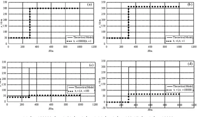
are unchanged. Four different weighting coefficients are applied to real and imaginary objective functions. The weights are λ1 =100000and λ2 =1, λ1=1 and λ2=1 , λ1=1 and λ2 =100 , λ1=1 and2 =100000
λ , respectively. The inversion results of zero-frequency resistivity and chargeability are shown from Figure 3 to Figure 4.
The second step: as can be seen from Figure 3 to Figure 4, the inversion results of zero-frequency resistivity and chargeability are the closest to the true values when weighting coefficients λ1=100000,λ2 =1 are used. Therefore, the
inversion results at this time are taken as the initial model values of zero-frequency resistivity and chargeability respectively and fixed, and began the second step to invert frequency dependence and time constant. Four different weighting coefficients, λ1=100000 and λ2=1 ,
1=1
λ
and λ2 =1 ,
1=1
λ and λ2 =100 ,
1=1
λ and
2 =100000
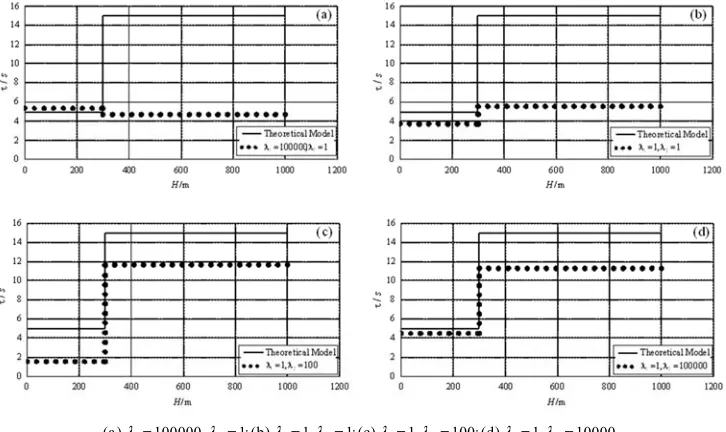
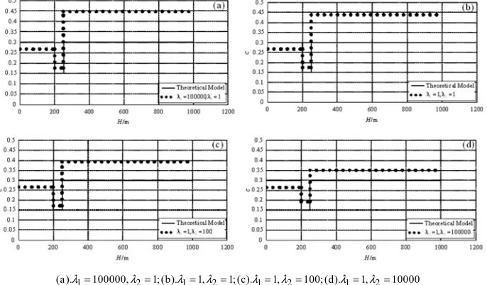
λ , are used in the second step inversion. The inversion results of frequency dependence and time constant are shown from Figure 5 to Figure 6.
When the weighting coefficient is λ1=100000,λ2 =1 in the first step inversion and the weighting coefficient is
1=1, 2=100000
λ λ in the second step inversion, the final fitting of the observation data and forward data is shown from Figure 7 to Figure 8.
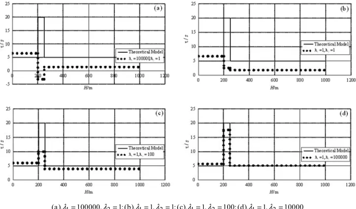
In Figure 3 to Figure 6, the abscissa is depth, and the ordinate is zero-frequency resistivity, chargeability, frequency dependence and time constant, respectively. In Figure 7 to Figure 8, the abscissa represents half of the length of the transmitter dipole AB, and the ordinate represents the real part and the imaginary part of the observation data (complex resistivity), respectively.
Figure 1. The inversion results of the resistivity of two layers polarization model with different initial models.
1 2 1 2 1 2 1 2
(a).λ =100000,λ =1; (b).λ =1,λ =1; (c).λ =1,λ =100; (d).λ =1,λ =10000
Figure 3. The inversion results of the resistivity of two layers polarization model with different weighting coefficients in the first initial model.
1 2 1 2 1 2 1 2
(a).λ =100000,λ =1; (b).λ =1,λ =1; (c).λ =1,λ =100; (d).λ =1,λ =10000
Figure 4. The inversion results of the chargeability of two layers polarization model with different weighting coefficients in the first initial model.
1 2 1 2 1 2 1 2
(a).λ =100000,λ =1; (b).λ =1,λ =1; (c).λ =1,λ =100; (d).λ =1,λ =10000
1 2 1 2 1 2 1 2
(a).λ =100000,λ =1; (b).λ =1,λ =1; (c).λ =1,λ =100; (d).λ =1,λ =10000
Figure 6. The inversion results of the time constant of two layers polarization model with different weighting coefficients in the first initial model.
Figure 7. The iterative fitting curve of real parts of complex resistivity when Hz.
Figure 8. The iterative fitting curve of imaginary parts of complex resistivity
when Hz.
Table 2. Polarization model of three layers.
parameters Zero-frequency resistivity chargeability time constant frequency dependence Layer thickness
ρ1 ρ2 ρ3 m1 m2 m3 τ1 τ2 τ3 m1 m2 m3 h1 h2 h3
true value 500 50 500 0.3 0.6 0.3 5 20 5 0.3 0.15 0.3 200 50 +∞
Initial 1 10 10 10 0.05 0.05 0.05 6 10 3.9 0.25 0.25 0.25 200 50 +∞
Fitting deference 0.1058
In the same way, four different weighting coefficients,
1=100000
λ and λ2 =1, λ1=1 and λ2 =1, λ1=1 and 2 =100
λ , λ1=1 and λ2 =100000 , are used to invert
zero-frequency resistivity and chargeability without changing the values of frequency dependence and time constant. The inversion results are shown in Figure 9 to Figure 10.
As can be seen from Figure 9 to Figure 10, the inversion results of zero-frequency resistivity and chargeability are the closest to the true values when weighting coefficients are
1=100000, 2 =1
λ λ used as the two-layer polarization model.
Therefore, the inversion results of zero-frequency resistivity and chargeability at the first step inversion of the three-layer polarization model are taken as the initial model values of zero-frequency resistivity and chargeability respectively, and unchanged, then the frequency dependence and time are
inverted. The inversion results are shown from Figure 11 to Figure 12.
When λ1=100000,λ2=1in the first-step inversion and
1=1, 2=100000
λ λ in the second inversion, the final fitting of the observation data and forward data is shown in Figure13 and Figure14. In Figure9~12, as in the case of the two-layer model, the abscissa represents depth and the ordinate represents the value of Cole-Cole parameters. In Figure 13~14, the abscissa represents half of the length of the emission dipole AB, and the ordinate represents the real part and the imaginary part of the apparent complex resistivity, respectively. From Figure 7 and Figure 8 and Figure 13~14, it can be seen that the real part and imaginary part of inversion observation data from two-layer and three-layer models fit well with forward data, and the fitting error is small.
0 0001
1 2 1 2 1 2 1 2
(a).λ =100000,λ =1; (b).λ =1,λ =1; (c).λ =1,λ =100; (d).λ =1,λ =10000
Figure 9. The inversion results of the resistivity of three layers polarization model with different weighting coefficients in the first initial model.
1 2 1 2 1 2 1 2
(a).λ =100000,λ =1; (b).λ =1,λ =1; (c).λ =1,λ =100; (d).λ =1,λ =10000
Figure 10. The inversion results of the resistivity of three layers polarization model with different weighting coefficients in the first initial model.
1 2 1 2 1 2 1 2
(a).λ =100000,λ =1; (b).λ =1,λ =1; (c).λ =1,λ =100; (d).λ =1,λ =10000
1 2 1 2 1 2 1 2
(a).λ =100000,λ =1; (b).λ =1,λ =1; (c).λ =1,λ =100; (d).λ =1,λ =10000
Figure 12. The inversion results of the time constant of three layers polarization model with different weighting coefficients in the first initial model.
Figure 13. The iterative fitting curve of real parts of complex resistivity when Hz.
Figure 14. The iterative fitting curve of imaginary parts of complex resistivity when f=0 0001. Hz.
It can be seen from Figure 3~4 and Figure 9~10 that the inversion results of zero-frequency resistivity and chargeability are different under different weighting coefficients. For two-layer and three-layer models, in the case of λ λ1≥ 2 , because the real part of apparent complex resistivity is larger than the imaginary part, the real part plays a major role in the inversion. The weighting coefficient
1=100000 2=1
λ ,λ makes the inversion results of
zero-frequency resistivity and chargeability slightly better
than that of weighting coefficientλ1=1,λ2 =1 (equal weight), but there is little difference. In the case of λ λ1< 2 , the imaginary part plays a larger role in the inversion, the inversion results of zero-frequency resistivity and chargeability are quite different from the true values, which can not reflect the trend of the models, and the vlue of chargeability appears negative.
The above analysis shows that the real part of apparent complex resistivity is more sensitive to zero-frequency resistivity and chargeability. When inverting zero-frequency resistivity and chargeability, the weighting coefficient of the real part λ1 should be larger than the weighting coefficient of the imaginary part λ2 in order to get better results.
As can be seen from Figure 5~6 and Figure 11~12, the inversion results of the frequency dependence and the time constant are different under different weighting coefficients. In the case of λ λ1≥ 2, the real part of apparent complex resistivity plays a major role in the inversion, and the inversion results of the frequency dependence and the time constant are worse than those when λ λ1< 2. For the two-layer model, when λ1=100000,
2 =1
λ , as shown in Figure 5(a) and Figure 6(a), the inversion results of the frequency dependence are worse than those of the other three weighting cases (the largest difference from the true values), while the inversion of the time constant does not get the results that can correctly reflect the original trend of the two-layer theoretical model, and the pseudo-extreme value appears at the depth of 300 m. When λ λ1= 2 =1, as shown in Figure 6(b), the inversion results of the time constant is not obvious. For the three-layer model, the inversion results of the frequency dependence can reflect the trend of the theoretical model when
1= 2 =1
λ λ , as shown in Figure 11(a) and Figure 12(b), but the error of the inversion results of the frequency dependence is the greatest compared with the other three weighting cases. The time constant appears obvious pseudo-extreme value at the depth of 200m. Whenλ λ1= 2 =1, as shown in Figure 11(b) and Figure
0 0001
12(b), the inversion results of the frequency dependence can reflect the trend of the three-layer model, but the error is larger than that when λ λ1< 2 . The inversion results of the time constant cannot reflect the original trend of the three-layer theoretical model correctly, and there is a pseudo-extreme value at the depth of 200 m.
When λ λ1< 2, the imaginary part of apparent complex resistivity plays an increasing role in the inversion, and the inversion results of frequency dependence and time constant can well reflect the original trend of the theoretical model. Compared with Figure 6(c), Figure 6(d), Figure 12(c) and Figure 12(d), the inversion results under λ1=1,
2 =100
λ
are slightly better than those under λ1=1,
2=100000
λ . It
is speculated that this is due to the fact that the imaginary part of apparent complex resistivity plays a greater role in the inversion when λ1=1,
2 =100000
λ . For the frequency dependence, we find that the inversion results under λ1=1,
2 =100
λ are slightly better than that under λ1=1 ,
2=100000
λ in the two-layer model when compared with the weights in Figure 5(c) and Figure 5(d). In the three-layer model, by comparing the inversion results of Figure 11(c) and Figure 11(d), we can also find that in the inversion results under λ1=1,
2 =100
λ , although the value of the last layer is slightly different from the true value, the first two layers are closer to the true value. It is not known that the inversion results of the frequency dependence are better with respect to that λ2 is larger than λ1.
The above analysis shows that the imaginary part of apparent complex resistivity is more sensitive to the frequency dependence and the time constant. λ2 the weighting coefficient of imaginary part of apparent complex resistivity should be larger than λ1 the real part of apparent complex resistivity to obtain better inversion results of the frequency dependence and the time constant.
3.2. Inversion Results and Analysis of 1D Weighting Inversion of Real and Imaginary Parts of SIP Data Containing the Regularization Constraint
Table 3 lists the values of the parameters of the theoretical model. The initial inversion model is assumed to be a polarized homogeneous half space. Using dipole-dipole device to collect data, a total of 100 arrays are arranged, each with a channel spacing of 5m, seven transmission frequencies: 0.00000001Hz, 0.0000000001Hz, 0.000001 Hz, 0.00001Hz, 0.0001Hz, 0.001 Hz, 0.01Hz, respectively. The real part and the imaginary part of the actual observation data are obtained by forward modeling. Four weighting coefficients are selected for weighting inversion. They are: λ1=100,λ2=1 ,
1=1 2 =1
λ ,λ ,
1=1 2 =100
λ ,λ and
1=1 2 =10000
λ ,λ .
The one by one inversion of Cole-Cole model parameters is used to reduce the multi-solution of inversion. The inversion is carried out in four steps, in order of zero-frequency resistivity, chargeability, frequency dependence and time constant.
In the first step, the zero-frequency resistivity is inverted
fixing chargeability, frequency dependenceand time constant unchanged (the initial value); in the second step, the zero-frequency resistivity obtained from the first inversion is taken as the initial value, and the chargeability is inverted fixing zero-frequency resistivity, frequency dependence and time constant unchanged; in the third step, the zero-frequency resistivity and chargeability obtained from the first two inversion steps are taken as the initial values. The frequency dependence are inverted fixing the zero-frequency resistivity, chargeability and time constant unchanged. In the fourth step, the zero-frequency resistivity, chargeability and frequency dependence obtained from the first three steps are taken as initial values, and the time constant is inverted fixing the zero-frequency resistivity, chargeability and frequency dependence unchanged. That is to say, the Cole-Cole model parameters obtained by the four-step inversion are zero-frequency resistivity, chargeability, frequency dependence and time constant.
Figure 15 (a), (b), (c), (d) are the inversion results of zero-frequency resistivity under four weighting coefficients respectively. Compared with the inversion results under
1=100 2=1
λ ,λ ,
1=1 2 =1
λ ,λ and
1=1 2=100
λ ,λ are
similar to each other, the inversion results under
1=100 2=1
λ , λ are closest to the theoretical model, and the
zero-frequency resistivity values of the first and third layers are relatively different from the theoretical model under
1=1 2=10000
λ ,λ .
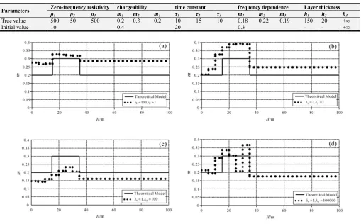
Figure 16 (a), (b), (c), (d) are the inversion results of chargeability under different weighting coefficients. The inversion results under λ1=100,λ2 =1can better reflect the shape of the theoretical model, but the values of the first and third layers are quite different from those of the theoretical model; the inversion results under λ1=1,λ2=1are similar to those under λ1=1,λ2 =100, and the inversion results under
1=1 2=10000
λ ,λ are closer to the theoretical model; when
1=1 2=10000
λ ,λ , there is a pseudo-extreme value in depth
of 25 m to 30 m.
Figure 17 (a), (b), (c), (d) are the inversion results of frequency dependence under four weighting coefficients respectively. The inversion results under λ1=100,λ2 =1 can reflect the shape of the theoretical model, but the value of the first layer is quite different from that of the theoretical model; the inversion results under λ1=1,λ2=1 and
1=1 2 =100
λ ,λ can not reflect the shape of the three-layer
model better. The inversion results under λ1=1,λ2 =10000 can better reflect the theoretical model, and the shape is closest to the theoretical model.
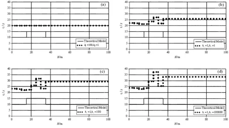
Figure 18 (a), (b), (c), (d) are the inversion results of time constant under four weighting coefficients respectively. The inversion results under λ1=100,λ2 =1 fail to converge, so the inversion results are a straight line. The inversion results under λ1=1,λ2=1,
1=1 2=100
Table 3. Polarization model.
Parameters Zero-frequency resistivity chargeability time constant frequency dependence Layer thickness
ρ1 ρ2 ρ3 m1 m2 m3 τ1 τ2 τ3 m1 m2 m3 h1 h2 h3
True value 500 50 500 0.2 0.3 0.2 10 15 10 0.18 0.22 0.19 150 20 +∞
Initial value 10 0.4 20 0.3 - - +∞
1 2 1 2 1 2 1 2
(a).λ =100,λ =1; (b).λ =1,λ =1; (c).λ =1,λ =100; (d).λ =1,λ =10000
Figure 15. The inversion results of the resistivity under different weighting coefficients.
1 2 1 2 1 2 1 2
(a).λ =100,λ =1; (b).λ =1,λ =1; (c).λ =1,λ =100; (d).λ =1,λ =10000
1 2 1 2 1 2 1 2
(a).λ =100,λ =1; (b).λ =1,λ =1; (c).λ =1,λ =100; (d).λ =1,λ =10000
Figure 17. The inversion results of the frequency dependence under different weighting coefficients.
1 2 1 2 1 2 1 2
(a).λ =100,λ =1; (b).λ =1,λ =1; (c).λ =1,λ =100; (d).λ =1,λ =10000
Figure 18. The inversion results of the time constant under different weighting coefficients.
4. Conclusion
On the premise of considering electromagnetic coupling, this paper studies the weighting inversion of real and imaginary parts of 1D spectrum induced polarization data, and draws the following conclusions:
1. The real part and imaginary part of apparent complex resistivity are sensitive to different Cole-Cole parameters. The
real part of apparent complex resistivity is sensitive to zero-frequency resistivity and chargeability. The imaginary part of apparent complex resistivity is sensitive to frequency dependence and time constant. The imaginary part of apparent complex resistivity is less sensitive to time constant than frequency dependence.
by fixing the values of frequency dependence and time constant unchanged. Then, the zero-frequency resistivity and chargeability obtained by the first step inversion are taken as the initial values of the second step inversion and fixed. Then, the frequency dependence and time constant are inverted. The feasibility of this method is verified by the trial calculation of theoretical model.
3. Using the weighting inversion of real and imaginary parts of apparent complex resistivity, the proportion of real and imaginary parts in inversion is controlled by weighting coefficients. Through model trial calculation, we find that the results under different weighting coefficients are different. When inversing zero-frequency resistivity and chargeability, we should add more weight to the real part, and when inversing frequency dependence and time constant, we should add more weight to the imaginary part. The algorithm can better invert the zero-frequency resistivity and chargeability, and effectively improve the inversion results of frequency dependence and time constant, and the results are more reliable.
References
[1] Ahmad Ghorbani, ChristianCamerlynck, NicolasFlorsch. 2009. CR1Dinv: A Matlab program to invert 1D spetral induced polarization data for the Cole–Cole model including electromagnetic effects. Computers&Geosciences 35 (2009) 255–266.
[2] Brown R J. 1985. EM coupling in multi-frequency IP and a generalization of the Cole-Cole impedancemodel. Geophysical prospecting, 33 (2): 282~302.
[3] Fan C S, Li T L, Yan J Y. 2012. Research and application experiment on 2.5D SIP inversion. Geophys. (in Chinese), 55 (12): 4044-4050.
[4] Ingeman-Nielsen, T, Baumgartner, F. 2006. CR1Dmod: a Matlab program to model 1D complex resistivity effects in electrical and EM surveys. Computers & Geosciences 32, 1411–1419.
[5] Liu B, Li S C, Li S C, et al. 2012. 3D electrical resistivity inversion with least-squares method based on inequality constraint and its computation efficiency optimization. Geophys. (in Chinese), 55 (1): 260-268.
[6] Liu S, Guan S Y, Gao PF. 1994. A polarization inversion method of Cole-Cole parameters of the polarizing sphere. Geophys. (in Chinese), 37 (S2): 542~551.
[7] Liu Y H, Yin C C. 2013. 3D inversion for frequency-domain HEM data. Chinese J. Geophys. (in Chinese), 56 (12): 4278-4287.
[8] Liu Y L, Li T L, Hu Y C, et al. 2015. Fast quasi-linear approximation and the three-dimensional spectrum of induced polarization inversion study. Geophys. (in Chinese), 58 (12): 4709-4717.
[9] Luo Y Z, Fang S. 1986. An approximate method to invert the spectrum of complex resistivity. Earth Science, 11 (1): 93-102. [10] Major J, Silic J. 1981. Restrictions on the use of Cole-Cole dispersion models in complex resistivity interpretation. Geo- physics, 46 (6): 916~931.
[11] Pelton W H, Ward S H, Hallof P G, et al. 1978. Mineral discrimination and removal of inductive coupling with multifrequency IP. Geophysics, 43 (3): 588~609.
[12] Sunde, E. D. 1968. Earth Conduction Effects in Transmission Systems. Dover, New York, p. 370.
[13] Shang T X. 2008. 1D full-region inversion of CSAMT of bipolar source [Master's Degree Thesis] (in Chinese). Changchun: Jilin University.
[14] Yu L B. 2010. The study of simulation and inversion of 1D spectrum induced polarization method [Master's Degree Thesis] (in Chinese). Changchun: Jilin University.
[15] Zhou F. 2015. 1D and 2.5D Modeling and Inversion of Complex Resistivity Data [Master's Degree Thesis]. East China institute of technology.