A Simulated Annealing Optimization Algorithm for Equal and Un-equal
Area Construction Site Layout Problem
N. Moradi, Sh. Shadrokh
Department of Industrial Engineering, Sharif University of Technology, Tehran, Iran.
A B S T R A C T
Construction Site Layout Planning (CSLP) is an important problem because of its impact on time, cost, productivity, and safety of the projects. In this paper, CSLP is formulated by the Quadratic Assignment Problem (QAP). At first, two case studies including equal and un-equal area facilities are solved by the simulated annealing optimization algorithm. Then, the obtained results are compared with the other papers. The comparisons show that the proposed Simulated Annealing (SA) is as efficient as ACO, PSO, CBO, ECBO, WOA, WOA-CBO, and ACO-PA which have been proposed by other papers for the same problems. As a result, the comparisons show that SA is as capable as other meta-heuristics of solving the combinatorial optimization problems like CSLP, while the hardware properties and computational times have been compared. Besides the comparisons, the design of experiments shows the relationship between each SA parameter and the computational time of the algorithm. Also, the history of convergence of the proposed SA indicates the high speed of reaching the optimal solution and the artificial intelligence of the proposed SA.
Keywords: Construction project, Construction site layout planning, Quadratic assignment problem, Simulated annealing.
Article history: Received: 28 November 2018 Revised: 13 February 2019 Accepted: 30 February 2019
1. Introduction
Problems which are related to construction projects consist of engineering design, cost estimation, planning, scheduling, and monitoring and control. Among these problems, planning is one of the most important phases because of its effect on time, cost, productivity, and safety of the projects. Furthermore, one of the most considerable cases in the planning stage is the site/floor layout [1]. Site layout or Construction Site Layout Problem (CSLP) deals with the determination of the locations of site-level facilities while considering the constraints of the project [2].
Corresponding author
E-mail address: [email protected] DOI:10.22105/riej.2019.169867.1073
International Journal of Research in Industrial
Locations of the facilities of CSLP can be modeled in two ways, discrete and continues. By discrete modeling, in which locations are represented as a single point or multiple points in a grid system, the computational complexity of the problem is getting lower. On the other hand, locations of continues modeling are not limited by distinct points, instead, they can be located in every place of the site. Also, in the discrete mode, if locations are considered predetermined and equal to the number of the facilities, the problem can be formulated by Quadratic Assignment Problem (QAP) - one of the hardest problems of operations research field - with assignment of one facility to each location exactly [3].
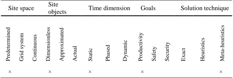
In the literature, CSLP had been investigated by many researchers over many years because of its important role in construction projects. By the review papers [4 and 5], the classification of CSLP, types of site space modeling, types of site layout objects, time dimension, types of objective functions, and optimization techniques were presented to solve the problem. Based on this mentioned classifications, the features of our paper problem is determined by sign × as it is given in Table 1. In Table 1, by predetermined location for site space, it means the locations considered for facilities are determined before and they are fixed. By dimensionless site objects, it means the dimensions of the facilities are considered one-dimension and as a geometry representation; they are just points. Static time means there is no change for material flows and the locations of the facilities are determined only one time. The goal of the objective function is about productivity because we consider the minimization of the material flow products distances between locations. Finally, the solution method of this paper is a meta-heuristics algorithm – simulated annealing.
Table 1. The features of the problem of our paper.
Site space Site
objects Time dimension Goals Solution technique
Pre d eter m in ed Gr id s y stem C o n tin u o u s Dim en sio n less Ap p ro x im ate d Actu al Static Ph ased Dy n am ic Pro d u ctiv ity Saf ety Secu rity E x ac t Heu ris tics Me ta -h eu ris tics × × × × ×
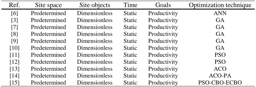
Table 2. References of the various scientific databases related to CSLP.
Ref. Site space Site objects Time Goals Optimization technique [6] Predetermined Dimensionless Static Productivity ANN
[3] Predetermined Dimensionless Static Productivity GA [7] Predetermined Dimensionless Static Productivity GA [8] Predetermined Dimensionless Static Productivity GA [9] Predetermined Dimensionless Static Productivity GA [10] Predetermined Dimensionless Static Productivity GA [11] Predetermined Dimensionless Static Productivity PSO [12] Predetermined Dimensionless Static Productivity PSO [13] Predetermined Dimensionless Static Productivity ACO [14] Predetermined Dimensionless Static Productivity ACO-PA [15] Predetermined Dimensionless Static Productivity PSO-CBO-ECBO
As it is shown in Table 2, GA is one of the popular optimization techniques that are used in the literature of CSLP. Now, we can state our motivation of this paper by the performed comparative study. In fact, by solving the numerical examples presented in each of these papers by our proposed technique, not only optimization algorithms can be compared with each other, but also the efficiency of the proposed algorithm to solve the various examples of CSLP can be shown. Moreover, CSLP with the class of problems, which are shown in Table 1, have never been solved by Simulated Annealing (SA) optimization algorithm which is the optimization technique of this paper. In the other words, in this paper, we are going to evaluate the SA parameters statistically by Design of Experiments (DOE) in order to investigate the relationship among SA parameters and the computational time of CSLP and the quality solution of the problem.
The main purpose of this article is to show the efficiency of SA algorithm of a solution of the combinatorial optimization problems like CSLP problem which is modeled by QAP formulation. In the following, in Section 2, SA is introduced briefly. In Section 3, the methodology of problem-solving based on SA is proposed. Next, in Section 4, the sample examples are solved and the results obtained by the proposed algorithm are compared with others’ findings. Finally, in the last section, conclusions have been mentioned.
2. Simulated Annealing Optimization Algorithm
3. Optimization of Construction Site Layout Problems using SA
3.1. Problem Definition
The construction site can be explained as the main building in which the goal of construction is to construct. This main building will be erected by using different facilities which will be located in the proper places around the main site. The determination of these locations of the facilities is the layout planning of the construction site. In other words, as a mathematical approach, CSLP can be formulated by QAP, which we want to detect the proper locations for the facilities. The case study with equal area facilities investigated in this paper is taken from [3], in which there are 11 facilities that have to be located in 11 predetermined locations in order to minimize the total travel distances among facilities. These 11 facilities are listed below:
Site office.
Falsework workshop.
Labor residence.
Storeroom 1.
Storeroom 2.
Carpentry workshop.
Reinforcement steel workshop.
Side gate.
Electrical, water, and other utility control room.
Concrete batch workshop.
Main gate.
Total construction space, which has the predetermined locations and its plan, is outlined in Figure 1. Also, the assumptions of this case study can be listed below:
All of the locations have the permission to accommodate each facility.
Locations are predetermined, and distances between locations had been calculated before.
The size of each facility is dimensionless.
Figure 1. Construction site of the case study mentioned by [3].
Now the mathematical model for the CSLP is formulated as below:
(1)
𝑀𝑖𝑛 𝑧 = ∑ ∑ ∑ ∑ 𝑥𝑖𝑘∗ 𝑥𝑗𝑙∗ 𝑓𝑖𝑗∗ 𝑑𝑘𝑙 𝑛
𝑘=1 𝑛
𝑙=1 𝑛
𝑗=1 𝑛
𝑖=1
(2)
∀𝑗 = 1,2, … , 𝑛 ∑ 𝑥𝑖𝑗
𝑛
𝑖=1 = 1
(3)
∀𝑖 = 1,2, … , 𝑛 ∑ 𝑥𝑖𝑗
𝑛
𝑗=1 = 1
(4)
∀𝑖, 𝑗 = 1,2, … , 𝑛 𝑖 ≠ 𝑗 𝑥𝑖𝑗 {0,1}
In this mathematical model, the objective function (1) is to minimize the total material flows among facilities products distances among locations. The notation 𝑥𝑖𝑗 is a binary variable (4), and
it takes one if the facility 𝑖 is allocated to location 𝑗. The notation 𝑓𝑖𝑗 indicates the frequency of the trips or flows between the facilities 𝑖 and 𝑗 per day. The notation 𝑑𝑖𝑗 indicates the distance between locations 𝑖 and 𝑗, and if there are more than one available paths between 2 facilities, the shorter distance will be considered. Also, 𝑛 is the number of facilities. It is noteworthy to say that in this model the number of locations should be equal to a number of facilities; otherwise, the “dummy” facilities with zero 𝑓 and 𝑑 will be added if the number of locations is more than the number of facilities. Moreover, constraints (2) and (3) control the assignment of only one facility to only one location.
3.2. Proposed SA
numbers are ordered in one arrow. For example, the first left number of the array will be an indicator of the first facility’s location and so the other facilities’ locations will be specified too. To clarify, one example of a representation of the solution space is shown in Table 3. Also, in Table 3, the solution space is just the second row, in which by changing the numbers of the locations, the solution space is searched along the feasible space. By this representation, which is indicated in Table 3, the process of searching solution space by the proposed algorithm will be fast. In this representation, the fixed facilities are considered easily by fixing the number of the fixed facility and are not permitted the other facilities to occupy those locations.
Table 3. Representation of the solution space of CSLP.
Facility 1 2 3 4 5 6 7 8 9 10 11 Location 3 5 1 8 7 2 11 10 6 4 9
In the following, the steps of the optimization algorithm based on SA are proposed. Input. Cooling schedule
𝑠 = 𝑠0 // the solution space is the permutation array of numbers 1 to 11
𝑡 = 0
𝑇0= 𝑇𝑚𝑎𝑥
Repeat
𝑘 = 0
Repeat
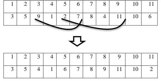
Generate neighbor solution by changing the mpair locations randomly (for example form=2)
1 2 3 4 5 6 7 8 9 10 11
3 5 9 1 2 7 8 4 11 10 6
1 2 3 4 5 6 7 8 9 10 11
3 5 4 1 6 7 8 9 11 10 2
∆𝐸 = 𝑓(𝑠)́ − 𝑓(𝑠)
If ∆𝐸 ≤ 0 then 𝑠 = 𝑠́
𝑘 = 𝑘 + 1
Until (𝑘 <epoch length)
𝑇𝑡+1= 𝛼 ∗ 𝑇𝑡 𝑡 = 𝑡 + 1
Until (𝑇𝑡 > 𝑇𝑚𝑖𝑛)
Output. Display the best solution.
In the above-mentioned pseudo-code, 𝑓(𝑠) is the objective function of the mathematical model,
𝑇𝑡 is the temperature of the SA at each stage 𝑡. In addition, the definition of each parameter of SA is given in Table 4. It is noteworthy to say that the parametermis considered in the experimental evaluation and its impact on the computational time and the quality of the solution is evaluated, so that if mis considered close to the size of the problem, the algorithm is only the stochastic searching process, and also if it is considered low, the algorithm cannot find the global solution or near to global solution.
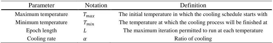
Table 4. Parameters of SA and each definition.
Parameter Notation Definition
Maximum temperature 𝑇𝑚𝑎𝑥 The initial temperature in which the cooling schedule starts with Minimum temperature 𝑇𝑚𝑖𝑛 The temperature at which the cooling process will be finished at Epoch length 𝐿 The maximum iteration permitted to run at each temperature
Cooling rate 𝛼 Ratio of cooling
4. Results and Discussion
In this section, at first, two case studies of construction site examined by other researchers were described, and the DOE of the SA parameters was done. The statistical analysis considered the relationship of SA parameters with both the execution time and solution quality of the problem. Then, by the results obtained from DOE and the statistical analysis, the optimal values of the SA parameters were determined. Finally, by the optimal SA parameters, two case studies (equal and unequal area) werre solved by the proposed SA. In the last part, the performance of the proposed SA was compared with a totally stochastic algorithm which generates the random solutions without any improvement at each iteration in order to evaluate the artificial intelligence of the proposed SA.
4.1. A Solution of the Equal Area Construction Site Layout Problem (EA-CSLP)
in Figure 2 for the frequency of the trips and distances between locations; these inputs are equal for 2 case studies.
Figure 2. Trip frequencies between facilities (left hand) and the distance between locations (right hand).
The descriptions of EA-CSLP are implied below:
In this problem, all of the locations are capable of accommodating each facility (equal area) and also there are 2 fixed facilities; facilities 8 and 11 must be located in the locations 1 and 10, respectively. In the following, DOE is performed and its result for investigating the relationship between SA parameters and the computational time is shown in Table 5. For the experiments,
𝑇𝑚𝑎𝑥 was valued by 1, 50, and 100; 𝑇𝑚𝑖𝑛 was valued by 0.1, 0.05, and 0.0001; 𝐿 was ranged by 5,
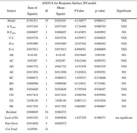
Table 5. Statistical analysis for investigating the relation between SA parameters and the computational time (EA-CSLP case study).
ANOVA for Response Surface 2FI model
Source Sum of
Squares
df Mean
Square
FValue p-value Significant
Model 0/391511 15 0/026101 6/136877 0/000412 YES
A-𝑇𝑚𝑎𝑥 0/073345 1 0/073345 17/24498 0/000749 YES
B-𝑇𝑚𝑖𝑛 0/000697 1 0/000697 0/163855 0/690992 NO
C-L 0/019734 1 0/019734 4/639971 0/046825 YES
D-α 0/093889 1 0/093889 22/07544 0/000242 YES
E-m 0/037813 1 0/037813 8/890591 0/008809 YES
AB 8/1E-05 1 8/1E-05 0/019045 0/89196 NO
AC 0/02387 1 0/02387 5/612446 0/030753 YES
AD 0/061752 1 0/061752 14/51938 0/001539 YES
AE 0/013456 1 0/013456 3/163816 0/094291 NO
BC 0/006972 1 0/006972 1/639337 0/218668 NO
BD 0/000506 1 0/000506 0/119031 0/734581 NO
BE 0/024649 1 0/024649 5/795549 0/028497 YES
CD 0/017424 1 0/017424 4/096784 0/059994 NO
CE 3/03E-05 1 3/03E-05 0/007112 0/933836 NO
DE 0/017292 1 0/017292 4/065807 0/060867 NO
Residual 0/068049 16 0/004253
Lack of Fit 0/053192 11 0/004836 1/627338 0/308371 not significant
Pure Error 0/014858 5 0/002972
Cor Total 0/45956 31
As it has been shown in Table 5, the parameters of 𝑇𝑚𝑎𝑥, 𝐿, 𝛼, and m are significant at the 0.05 level. So, we can conclude by the results of Table 5 that the computational time is affected by
Table 6. Optimal values for minimization of the computational time of EA-CSLP case study.
Parameter Optimal value by DOE
𝑇𝑚𝑎𝑥 1
𝑇𝑚𝑖𝑛 0.0001
𝐿 10
𝛼 0.99
M 4
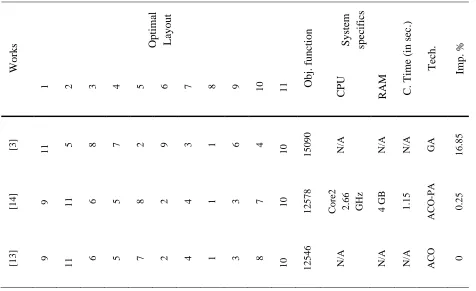
In the following, the result of solution of EA-CSLP case study by the proposed algorithm with its optimal parameters is shown in Table 7, and also the comparison of the results with the other works is indicated. For EA-CSLP, the proposed algorithm gained the better objective function value than two first algorithms, and also the proposed SA was as efficient as ACO, PSO, CBO, ECBO, WOA, and WOA-CBO which had been proposed by other papers of the solution of EA-CSLP example. In Table 7, Imp% is calculated by (the best solution by this paper-the best solution by the other works) the best solution by the other works.
Table 7. A comparison between the results of the current work and previous papers in EA-CSLP case study.
Wor
k
s Opt
im al Layout O bj . f un ct ion Syst em spe ci fi cs C . Tim e ( in s ec .)
Tech. Imp.
%
1 2 3 4 5 6 7 8 9 10 11
C
PU
RAM
[3
]
11 5 8 7 2 9 3 1 6 4 10 150
9
0
N/A N/A N/A GA 16.8
5
[1
4
]
9 11 6 5 8 2 4 1 3 7 10
1 2 5 7 8 C o re2 2 .6 6
GHz 4 GB 1.1
5 AC O -PA 0 .2 5 [1 3 ] 9
11 6 5 7 2 4 1 3 8 10 125
4
6
N/A N/A N/A AC
O
Wor
k
s Opt
im al Layout O bj . f un ct ion Syst em spe ci fi cs C . Tim e ( in s ec .)
Tech. Imp.
%
1 2 3 4 5 6 7 8 9 10 11
C PU RAM [1 5 ] 9
11 5 6 7 4 3 1 2 8 10 125
4 6 C o re7 1 .7 3
GHz 4 GB N/A PSO 0
[1
5
]
9
11 6 5 7 4 3 1 2 8 10 125
4 6 C o re7 1 .7 3
GHz 4 GB N/A CBO 0
[1
5
]
9
11 4 5 7 6 3 1 2 8 10 125
4 6 C o re7 1 .7 3
GHz 4 GB N/A EC
B O 0 [1 9 ] 9
11 4 5 7 6 3 1 2 8 10 125
4 6 C o re7 1 .7 3
GHz 4 GB N/A W OA 0
[1
9
]
9
11 4 5 7 6 3 1 2 8 10 125
4 6 C o re7 1 .7 3
GHz 4 GB N/A WOA
-CBO 0 C u rr en t wo rk 9
11 5 6 7 2 4 1 3 8 10 125
4 6 C o re3 2 .3 0
GHz 2 GB 0.0
0
6
SA -
4.2. The Solution of the Un-equal Area Construction Site Layout Problem (UA-CSLP)
Second case study (UA-CSLP) is taken from [7]. In this problem, all of the locations are not capable of accommodating each facility (un-equal area); unlike the previous problem, the facilities 1, 3, and 10 cannot be located in the locations 7 and 8.
points in order to investigate the relationship between each SA parameters and the computational time. Also, at the experiments of UA-CSLP, the relation between SA parameters and the solution quality were not investigated, because most of the experiment points reached the optimal solution.
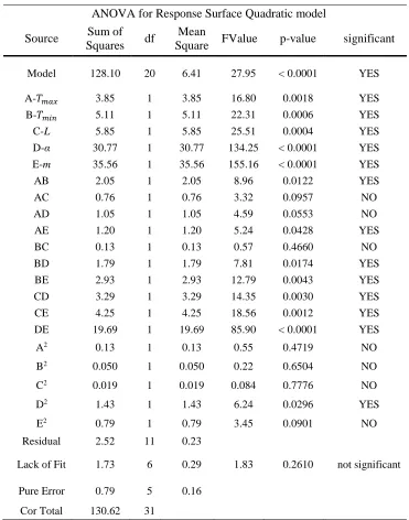
Table 8. Statistical analysis for investigating the relation between SA parameters and the computational time (UA-CSLP case study).
ANOVA for Response Surface Quadratic model
Source Sum of Squares df
Mean
Square FValue p-value significant
Model 128.10 20 6.41 27.95 < 0.0001 YES
A-𝑇𝑚𝑎𝑥 3.85 1 3.85 16.80 0.0018 YES
B-𝑇𝑚𝑖𝑛 5.11 1 5.11 22.31 0.0006 YES
C-L 5.85 1 5.85 25.51 0.0004 YES
D-α 30.77 1 30.77 134.25 < 0.0001 YES
E-m 35.56 1 35.56 155.16 < 0.0001 YES
AB 2.05 1 2.05 8.96 0.0122 YES
AC 0.76 1 0.76 3.32 0.0957 NO
AD 1.05 1 1.05 4.59 0.0553 NO
AE 1.20 1 1.20 5.24 0.0428 YES
BC 0.13 1 0.13 0.57 0.4660 NO
BD 1.79 1 1.79 7.81 0.0174 YES
BE 2.93 1 2.93 12.79 0.0043 YES
CD 3.29 1 3.29 14.35 0.0030 YES
CE 4.25 1 4.25 18.56 0.0012 YES
DE 19.69 1 19.69 85.90 < 0.0001 YES
A2 0.13 1 0.13 0.55 0.4719 NO
B2 0.050 1 0.050 0.22 0.6504 NO
C2 0.019 1 0.019 0.084 0.7776 NO
D2 1.43 1 1.43 6.24 0.0296 YES
E2 0.79 1 0.79 3.45 0.0901 NO
Residual 2.52 11 0.23
Lack of Fit 1.73 6 0.29 1.83 0.2610 not significant
Pure Error 0.79 5 0.16
Cor Total 130.62 31
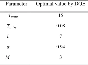
Table 8, we can say that the lack of fit of the model is insignificant, so the quadratic model fits correctly and the results are valid. By the help of DOE, the optimal values of the parameters of SA are obtained, as it is shown in Table 9. These optimal values minimize the computational time of UA-CSLP case study.
Table 9. Optimal values for minimization of the computational time of UA-CSLP case study.
Parameter Optimal value by DOE
𝑇𝑚𝑎𝑥 15
𝑇𝑚𝑖𝑛 0.08
𝐿 7
𝛼 0.94
M 3
Table 10. A comparison between the results of the current work and previous papers in UA-CSLP case study. W o rk s Op tim al L ay o u t Ob j. Fu n ctio n Sy stem s p ec if ic C . tim e (s ec .) T ec h . Im p . %
1 2 3 4 5 6 7 8 9 1 0 1 1 C P U R A M
[7
]
11 5 9 7 2 8 3 1 6 4 10
1
5
1
6
0
N/A N/A N/A GA 16.8
4
[1
9
]
11 9 5 6 8 3 7 1 4 2 10
1 2 6 0 6 C o re7 1 .7 3
GHz4 GB N/A W
OA 0
[1
9
]
11 9 5 6 8 3 7 1 4 2 10
1 2 6 0 6 C o re7 1 .7 3
GHz4 GB N/A WOA
- C BO 0 [1 4 ]
11 9 6 5 8 3 7 1 4 2 10
1 2 6 0 6 C o re2 2 .6 6
GHz4 GB 1.1
5 AC O -PA 0 C u rr en t W o rk
11 9 6 5 8 3 7 1 4 2 10
1 2 6 0 6 C o re3 2 .3 0
GHz2 GB 0.2
1
SA -
Figure 3. Comparison of convergence of SA with the totally stochastic algorithm of UA-CSLP case study (vertical axis: objective function value, horizontal axis: iterations).
5. Conclusions
In this paper, we solved two case studies namely EA-CSLP and UA-CSLP in the literature related to CSLP. After executing DOE, optimal values of SA parameters were obtained and then the results of the solution of the case studies were compared with the other algorithms proposed by other researchers. The comparisons showed the efficiency of the proposed algorithm of the discrete CSLP examples, also SA was as capable as other meta-heuristics of solving the combinatorial optimization problems like CSLP problem, while the hardware properties and computational times were compared because in this paper CSLP was formulated by QAP. Furthermore, the experiments showed the relationship between each parameter and the performance of the algorithm, for example, the parameters 𝑇𝑚𝑎𝑥, 𝐿, 𝛼 and m, were significant at both example, especially 𝛼 and m were distinguished significant, so that they had impact on the computational time significantly. Finally, the history of convergence of the proposed SA showed the high speed of reaching to the optimal solution, also the artificial intelligence of the proposed SA to reach the best solution, while it was executed by the system with the low RAM and not strong CPU. For future studies, it is recommended to solve the other case studies of CSLP like continues examples by the proposed SA. Also, the efficiency of the proposed algorithm can be assessed by solving the dynamic time (DCSLP) problems which are more complicated and comparisons will be better in these cases.
References
Liao, T. W., Egbelu, P. J., Sarker, B. R., & Leu, S. S. (2011). Metaheuristics for project and construction management–A state-of-the-art review. Automation in construction, 20(5), 491-505. Li, H., & Love, P. E. (2000). Genetic search for solving construction site-level unequal-area facility layout problems. Automation in construction, 9(2), 217-226.
10000 11000 12000 13000 14000 15000 16000 17000 18000
0 50 100 150
SA
Li, H., & Love, P. E. (1998). Site-level facilities layout using genetic algorithms. Journal of computing in civil engineering, 12(4), 227-231.
Andayesh, M., & Sadeghpour, F. (2014). The time dimension in site layout planning. Automation in construction, 44, 129-139.
Sadeghpour, F., & Andayesh, M. (2015). The constructs of site layout modeling: an overview. Canadian journal of civil engineering, 42(3), 199-212.
Yeh, I. C. (1995). Construction-site layout using annealed neural network. Journal of computing in civil engineering, 9(3), 201-208.
Li, H., & Love, P. E. (2000). Genetic search for solving construction site-level unequal-area facility layout problems. Automation in construction, 9(2), 217-226.
Tam, C. M., Tong, T. K., & Chan, W. K. (2001). Genetic algorithm for optimizing supply locations around tower crane. Journal of construction engineering and management, 127(4), 315-321.
Tam, C. M., Tong, T. K., Leung, A. W., & Chiu, G. W. (2002). Site layout planning using nonstructural fuzzy decision support system. Journal of construction engineering and management, 128(3), 220-231.
Cheung, S. O., Tong, T. K. L., & Tam, C. M. (2002). Site pre-cast yard layout arrangement through genetic algorithms. Automation in Construction, 11(1), 35-46.
[11] H. Zhang, J.Y. Wang, Particle swarm optimization for construction site unequal-area layout, Journal of construction engineering and management, 134 (2008) 739-748.
Lien, L. C., & Cheng, M. Y. (2012). A hybrid swarm intelligence based particle-bee algorithm for construction site layout optimization. Expert systems with applications, 39(10), 9642-9650.
Gharaie, E., Afshar, A., & Jalali, M. R. (2006, February). Site layout optimization with ACO algorithm. Proceedings of the 5th WSEAS international conference on artificial intelligence, knowledge engineering and data bases (pp. 90-94). World Scientific and Engineering Academy and Society (WSEAS).
Calis, G., & Yuksel, O. (2015). An improved ant colony optimization algorithm for construction site layout problems. Journal of building construction and planning research, 3(04), 221.
Kaveh, A., Khanzadi, M., Alipour, M., & Moghaddam, M. R. (2016). Construction site layout planning problem using two new meta-heuristic algorithms. Iranian journal of science and technology, transactions of civil engineering, 40(4), 263-275.
Kirkpatrick, S., Gelatt, C. D., & Vecchi, M. P. (1983). Optimization by simulated annealing. science, 220(4598), 671-680.
Abbasi, B., Shadrokh, S., & Arkat, J. (2006). Bi-objective resource-constrained project scheduling with robustness and makespan criteria. Applied mathematics and computation, 180(1), 146-152. Park, M. W., & Kim, Y. D. (1998). A systematic procedure for setting parameters in simulated annealing algorithms. Computers & operations research, 25(3), 207-217.
![Figure 1. Construction site of the case study mentioned by [3].](https://thumb-us.123doks.com/thumbv2/123dok_us/8580075.1718723/5.612.177.439.100.275/figure-construction-site-case-study-mentioned.webp)