Data Augmentation and Bayesian Methods for Multicategory Support Vector Machines

http://www.sciencepublishinggroup.com/j/ijdsa doi: 10.11648/j.ijdsa.20190503.12

ISSN: 2575-1883 (Print); ISSN: 2575-1891 (Online)

Data Augmentation and Bayesian Methods for

Multicategory Support Vector Machines

Yeqian Liu

Department of Mathematical Sciences, Middle Tennessee State University, Murfreesboro, USA

Email address:

To cite this article:

Yeqian Liu. Data Augmentation and Bayesian Methods for Multicategory Support Vector Machines. International Journal of Data Science and Analysis. Vol. 5, No. 3, 2019, pp. 42-51. doi: 10.11648/j.ijdsa.20190503.12

Received: June 30, 2019; Accepted: July 24, 2019; Published: August 7, 2019

Abstract:

The support vector machine (SVM) has become very popular within the machine learning literature. Recently, SVM has received much attention from statisticians. It is well known that for multicategory classification problem, the commonly used multicategory SVM is based on the frequentist framework. In this paper, we develop a multi-class support vector machine under the Bayesian framework. Numerical studies were performed by EM and the Bayesian algorithm Gibbs sampler. Our results have shown that the classification accuracy of the Bayesian approach is comparable to that of frequentist approaches, while Bayesian approach also has the advantage of providing estimates of uncertainty in predictions.

Keywords:

Multivariate Classifcation, MSVM, MCMC, EM

1. Introduction

Recently, Support vector machine has drawn attention from the statistics community during the high popularity of SVM rising in machine learning literature. The well-known two category SVM for the binary classification problem can be interpreted geometrically with a hyperplane which gives the maximum margin of discriminating one class from the other. See Boser, Guyon, & Vapnik [1], Vapnik [2], and Burges [3]. In two category SVM, the separation is achieved by a hyperplane which has the largest distance to the data of the two groups.

Bayesian approach, which has been developed rapidly during the past thirty years, plays a very important role in statistics. Nicholas G and Steven L [4] applied the Bayesian approach to SVM classification problem. In their paper, they developed a latent variable representation of original SVM, which enable to use EM or MCMC algorithms do parameter estimation. In their method, data augmentation methods can be formulated in terms of complete data sufficient statistics, which is a considerable advantage when working with large data sets, where most of the computational expense comes from repeatedly iterating over the data. Methods based on complete data sufficient statistics need only compute those statistics once per iteration, at which point the entire parameter vector can be updated. [4]

Recently, it was shown that the support vector machine (SVM) [5] admits a Bayesian interpretation through the technique of data augmentation. However, existing inference methods for the Bayesian support vector machine [6] can only handle two-category classification problem under Bayesian framework. Based on stochastic variational inference [7] and inducing points [8], we develop a Bayesian support vector machine for multicategory classification problem in this paper. The proposed Bayesian multicategory SVM not only inherits the advantage of robustness against outliers, advanced accuracy [9], and guaranteed error rate [10] from the frequentist formulation of the SVM, but like all Bayesian methods, it also has the advantage of modeling with high flexibility, automatic parameter tuning, and providing estimates of uncertainty in predictions.

This article is organized as follows. Section 2 states the loss function and Bayesian models for multi-SVM. Section 3 describe the Point estimation by EM and other related algorithms. Section 4, present the MCMC for SVM. Finally, Section 5 gives concluding remarks and discussion of future directions.

2. Multicategory Support Vector

Machines

binary case based on a k-dimensional predictors,where the class labels are either 1 or -1. And the -norm regularized support vector classifier seeks minimizing:

∑ max(1 − , 0) + ∑ | / | (1)

where is the standard deviation of the ’th predictor variable, except that = 1 for the intercept term, and is a tuning parameter. [11]

2.1. Model and Notations

In this section, we will extent this model to the multicategory case. Consider a k-category classification problem with a vector of predictors = (1, , . . . , _" ). Class labels are defined as follows. If example # falls into class , then is equal to a k-dimensional vector with 1 in the -th coordinate and −1/($ − 1) elsewhere. Accordingly, define a % − $ function &( ) = (& ( ), . . . , & ( )), for any

∈ ℝ"_{. Where &}

)( ) = ) for r=1,...,k. Let be a $ − $

function that maps to a k-dimensional vector with 0 in the ’th coordinate and 1 elsewhere, if example i is in class j. Now, we propose an extension of support vector classifier to choose a set of coefficients to minimize:

* ( , ) = ∑ ( ) × (&( ) − , )-+ ∑ ) ∑ " | )/ | (2)

The scaling variable is the standard deviation of the -th predictor variable, except that =1 for the intercept term. And is a tuning parameter. It can be shown that minimizing (2) is equivalent to maximize the following pseudo-posterior density

%( | , ., ) ∝ 0 %{−* ( , 2)}

∝ 4 ( ) ( | )%( | , .) (3)

where 4 ( ) is a pseudo-posterior normalization constant. The pseudo-likelihood ( | ) can be written as

( | ) = ∏ ( | ) = exp{−2 ∑ ( ) × (&( ) − )-} (4) For simplicity, define 9₎( ) = (&₎( ) − ₎), then

( ) × (&( ) − )-= ∑) ,): ;< (9)( ),0) (5)

if example i is from class j.

Therefore, the pseudo-likelihood for example # is rewritten as

( | ) = exp=−2 ∑) ,): max(9)( ),0)>

= ∏) ,): 0 %{−2max(9)( ),0)}

= ∏) ,): ? _{A BCDE}@ _FGexp H−(IG(JF)-EFG) K CEFG L *M)

(6)

The last step is from Theorem in [12] where M is a vector of latent variables paired with .

Denote N as the class label of example i, then the pseudo-likelihood can be rewritten as

( | ) = ∏ ( | ) = ∏ ∏) ,):OF?

@

A BCDEFGexp H− (IG(JF)K

CEFG L *M)

= ∏ ∏) ? A@PBCDEFGexp H− (IG(JF))K

CEFG LQ R(OF:))

(7)

Based on the objective function in (2), consider the exponential power prior distribution for which contains the regularization penalty as follows

%( | , .) = ∏) ∏ " %( ) | , .) = ∏) H_{ST( -} UV₎L

"

exp W− ∑ " XYGZ

S[ZX \ (8)

In general, consider . ∈ (0,2] where . = 2 corresponds to the “ridge regrssion" and . = 1 corresponds to the “lasso". Then the prior regularization penalty can be expressed as a scale mixture of normals.

%( ) | , .) = ? _A@^( ) |0, C_) C)%(_)|.)*_) (9) where %(_₎ |.) is exponential with mean 2 for the special case of . = 1.

2.2. Conditional Distribution

According to the above computations, especially equations (7) and (9), the support vector machine pseudo-posterior distribution can be expressed as the marginal of the complete data pseudo-posterior distribution as follows:

%( , M, _| , , .) ∝ ∏ ∏) PM)A.`exp W−(JF

a_{YG bFG-EFG)}K

CEFG \Q

R(OF:))

× ∏) ∏ " _)A.`exp W− YGZ

K

CSK_cGZ[ZK\ %(_) |.)

(10)

Define d ₎≜ {#: N ≠ h} as the set of all subjects who does not fall in class r. Rewrite the complete data pseudo-posterior distribution as

%( , M, _| , , .) ∝ ∏) ∏∈iUGM)A.`exp W−

(J_FaYG bFG-EFG)K

CEFG \

× ∏) ∏ " _)A.`exp W− YGZ

K

CSK_cGZ[ZK\ %(_)|.)

(11)

The full conditional distribution of given M, _,

%( )| , M), _), ) ∝ ∏∈iUG ∏ " exp W−

(J_FaYG bFG-EFG)K

CEFG \ × exp W−

Y_GZK

CSK_cGZ[ZK\ (12)

Define the matrices Λ₎= *#<k(M₎), Ω₎= *#<k(_₎) , where the diagram elements of Λ₎ and Ω₎ are the elements of M₎ and _₎, respectively. And = *#<k( C, . . . , _"C). Also let m₎ denote a matrix with row # equal to, , the predictor vector of the #’th subject in Θ ₎.

This model can be written in hierarchical form:

)− M)= m) )+ ΛC)oEG

)= 1Ω)CΣCoYG

where oYG and oEG are vectors of iid standard normal deviates with dimensions matching ₎ and M₎.

Thus, for ₎ has a conditional normal posterior distribution given by:

%( )| , M), _), ) ∼ r(s), t)) (13)

where =

t) = C _) + m)Λ) m) <u* s)= t)m)( )× M) − 1) (14)

The full conditional distribution for M₎ and _₎ given

, , Consider the conditional distribution of M₎ for r=1,..,k and # ∈ Θ ₎ . Note that from the complete pseudo-posterior distribution we can get:

%(M)| ), )) ∝ 1

B2vM)exp w− 1

2 x( )− ))

C

M) + M)yz

∼ {ℐ{ }1_{2 , 1, (} )− ))C~

This implies that:

(M)| ), )) ∼ ℐ{(| )− )| , 1) (15)

For the full conditional distribution of _₎ , it is proportional to the integrand in equation (9). In general this is

complicated because its prior density %(_₎|.) is generally not available. However, for the two special cases of . = 1 and . = 2 closed from solutions are available. When

. = 2, %(_)| ) ) is a point mass at 1. For . = 1, the full conditional distribution of _₎ is:

%(_) | ) , ) ∝ 1

B2v_) exp w− 1 2 x )

C_/ C C

_) + _) yz

∼ {ℐ{ x1_{2 , 1, C C})C )y

Thus similarly

(_) | ) , ) ∼ ℐ{( /| )|,1) (16)

Later we will use these distributions to develop learning algorithms.

3. Point Estimation by EM and Other

Related Algorithms

In this section, we use the distributions obtained in Section 2 to construct EM-style algorithms to estimate the coefficients. First, an EM algorithm for learning with a fixed value of the tuning parameter is developed. Then we develop an ECME algorithm to learn and simultaneously.

3.1. Learning • with Fixed €

With the augmented data M and _, the EM algorithm is a iterative method for finding posterior modes or MLEs. From equation (12), we know that the posterior distribution of the

)’s for r=1,...,k are independent. So we can estimate them

separately using the EM algorithm. For ₎, the E-step and M-step are defined by

• − ‚ƒ0% „( )| )(…)) = ? log%( )| , M), _), )%(M), _)| )(…), ‰, )*M)*_)

Š − ‚ƒ0% )(…- ) = argmax_YG „( )| )(…)) (17)

Note that any term in log%( ₎| , M₎, _₎, ) that is free of

) can be absorbed to the constant. This leaves us only the linear function of M₎ and _₎ . Thus, we only need to replace them with their conditional expectations MŒ₎(…) and _•₎ (…) for the calculation of function „( ₎| ₎(…)), given ₎ and the observed data.

As we discussed before, the result for _₎ would depend on the value of .. Focus on the case where . = 1. And according to equation (16), we can obtain that:

_) (…)= | ) |

Recall that the conditional posterior of _Ž follows a multivariate normal distribution. Thus, the posterior mode

will be the same as the posterior mean. By equations (13) and (14), we can get the following algorithm.

Algorithm: EM-SVM

Repeat the following until convergence

E-Step Given a current estimate ₎= ₎(…), compute:

MŒ₎(…)= | )− )| , Λ•) (…)= *#<k•MŒ) (…)‘, Ω•) (…)= *#<k•_•) (…)‘,

)(…- )= H CΣ Ω•) (…)+ m)Λ•) (…)m)L m)( )× MŒ) (…)− 1)

3.2. Learning • and € Simultaneously

In order to learn and 2 together, the generalized expectation-conditional maximization algorithm (ECME) is used, where the last“E" represents the conditional maximization of either function. To implement the ECME

algorithm, we assume a inverse gamma prior distribution for :

%( ) ∝ ( ) ’ exp(−s_S )

Combine this prior with equation (8), we can find the conditional posterior density of given and .

%( | , .) ∝ ( )" - ’ _{exp “− ”s}

S+ •

) •

"

– )– —˜

The following algorithm can be obtained with minor modification of the EM-SVM algorithm.

Algorithm: ECME-SVM

E-Step Identical to the E-step of EM-SVM with = (…). CM-Step Identical to the M-step of EM-SVM with

= (…)_.

CME-Step Set

( )(…- )₌sS+ ∑) ∑" | ) (…)_{/ |}

%$/. + <S− 1

4. Fully Bayesian Multicategory Support

Vector Machines

In the MSVM framework of [15], following [12, 13], we can find f(. ) by minimizing the following penalized function when . = 1,

*(β, ) = ∑ L(y ) ⋅ (f(x ) − y )-+ ∑) ∑" |Y_[GZ_Z| (18)

or equivalently,

*(β, ) = ∑) ∑∈⊝UG(&)(x ) + )-+ ∑) ∑ " |

YGZ

[Z| (19)

with constraints ∑₎ &₎(Ÿ ) = 0 for # = 1, ⋯ , u.

where is the standard deviation of the ′element of Ÿ, is a tuning parameter and ⊝ ₎= {#: N ≠ h} , N is the classification number of observation #.

The minimization problem (19) can be viewed to find the mode of pseudo-posterior distribution from the Bayesian perspective. That is

%(β| , y) ∝ exp(−*(β, )) ∝ 4( ) (y|β)%(β| ) (20) where 4( ) is a normalization constant. According to the form of the objective function, we can adopt the following likelihood function for the data and assume a exponential power prior for β as follows;

(y|β) = ∏ ( |β) = exp{−2 ∑ L(y ) ⋅ (f(x ) − y )-} (21)

%(β| ) = ∏) ∏ " %( )| ) = (∏) ∏ " _CS[Z)exp(− ∑) ∑ " |Y_S[GZ_Z|) (22)

where [ ₎| ] follows the Laplace distribution.

Now,following [14], we assume a gamma prior on , i.e.

%( ) ∝ ( )£’ exp(−s_S ) ₍₂₃₎

with hyper-parameters (<_S, s_S). Then we use the independent Jeffreys noninformative prior, called the invariance prior, on

,

%( ) ∝_[

Z (24)

for = 1, ⋯ , %.

Theorem 1 Under the penalized function (19) and the priors (23) and (24), following the data augmentation approach proposed by [15], we have the following full conditional posterior distributions

[β)| , λ), w), y] ∼ r(b), B)) (25) [M)|β), )] ∼ ℐ{(|x β)− )| , 1) (26)

[¨) | ) , , ] ∼ ℐ{( /| ) |,1) (27)

[ |β, ] ∼ Gamma(%$ + <S− 1, sS+ ∑) ∑" |Y_[GZ_Z|) (28)

[ | , β] ∼ Inv. Gamma($,_S∑) | )|) (29)

for # ∈⊝ ₎; h = 1, ⋯ , $ and = 1, ⋯ , %. Where B₎ =

C_{Σ Ω}

) + X)Λ) X) and b)= B)X)Λ) (y)− λ)). And y)= { )}∈⊝UG, λ)= {M)}∈⊝UG, Λ)= *#<k(λ)) , Ω)=

*#<k({¨) }" ), Σ = *#<k({ C}" ), 1 is the vector of 1’s. X) is a matrix with row # is , # ∈⊝ ).

Then the MCMC algorithm is developed from Theorem 1. Algorithm: MCMC-MSVM

Draw β₎(…- ) from r(b₎(…), B₎(…)) for h = 1, ⋯ , $; Draw M₎(…- ) from ℐ{(|x β₎(…- )− ₎| , 1) independently, for h = 1, ⋯ , $; # ∈⊝ ₎;

Draw ¨₎ (…- ) from ℐ{( (…) (…)/| ₎(…- )|,1) independently, for h = 1, ⋯ , $ and = 1, ⋯ , %;

Draw (…- ) from Gamma(%$ + <_S− 1, s_S+

∑) ∑ " |YGZ

(¯°V)_|

Draw (…- ) from Inv. Gamma $,_S¯°V ∑₎ | ₎…- |

for 1, ⋯ , %.

5. Application

5.1. Data Introduction

TIMSS represents the Trends in the International Mathematics and Science Study, which is one of the most important and largest global studies in education achievement. TIMSS was first conducted in 1995, and it collected data every four years on the achievement of fourth and eighth grade students internationally. TIMSS 2011 is the fifth in the series of assessments. 32 countries participated in the TIMSS 2011 assessments. There is enormous diversity among the TIMSS countries—in terms of economic development, geographical location, and population size. Countries participating in TIMSS aim for a sample of at least 4,500 students to ensure that there are enough respondents for each item. This study dedicates to improving teaching and learning in mathematics and science by comparing different country and exploring the environmental factors that predict students’ achievement.

The TIMSS 2011 International Database includes the data from instruments that were administered to the students, their parents, their teachers, and their school principals. These include the student responses to the achievement items:

TIMSS mathematics and science and students, teacher and principals’ responses to the student, home, teacher, and school background questionnaires. This is a large dataset with six files in it: school background data files, student background data files, student achievement data files, home background data files, student-teacher linkage files and teach background data files.

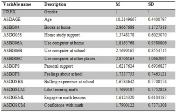
We used the 4²³ grade USA data in the dataset. 12569 U.S students participated in this study. Students were administered a background questionnaire with questions related to their home background, school experiences, and attitudes toward reading, mathematics, and science. An example question is “About how many books are there in your home? (Do not count magazines, newspapers, or your school books.” The student background data files contain students’ responses to these questions. It includes 15 variables. Each variable may have multiple items. For example, mathematics self-concept has 7 items. We will use the mean of the items of a variable as the score. Except those questions especially designed for learning science, 13 potential predictors from the student background data files were used in the model. There are two demographic variables: sex and age; six environmental variables about recourses and parental support; five psychological variables about students; feeling and experiences. Figure 1 shows the description of the predictors and their descriptive statistics.

Figure 1. Predictors and descriptive statistics.

Figure 3. Percent of each group.

Since the data we used are from the U.S which is a developed country, some of the measures might be skewed or reaching a celling effect. For example, ASBG05S ranges from 0 to 2 with a mean at 1.57. It is negatively skewed.

The predictor is student’s achievement level. Students of highest achievement are in group 5 which the students of the lowest achievement are in group 1. Figure 2 and 3 shows the frequency and percent of each group.

5.2. Traditional Methods

Before applying the new method, three traditional methods were used to classify the current data.

Firstly, we used Linear Discriminant Analysis (LDA). Two types of prior were used: proportional and equal. The results showed that when proportional prior were used, the total error rate was 57.67%. The error count estimates were highest at the two ends. For group 1 and group 5, then error rate were both larger than 90%, while for group 3 and group 4, the error rates were about 40%. When equal prior were used, the total error rate was 62.16%, but the error rate were highest in the middle groups (all three groups had an error rate that was larger than 75%). The error rates at the ends were smaller, 47.80% for group1 and 34.62% for group 5.

Secondly, apply QDA on this data. As LDA, Two types of prior were used: proportional and equal. The results showed that when proportional prior were used, the resubstitution error rate was 56.23%. The error count estimates were highest at group1 (95%), while for group 3 and group 4, the error rates were about 50%. When equal prior were used, the total error rate was 58.76%, but the error rate were highest in the middle groups (all three groups had an error rate around 70%). The error rates at the ends were smaller, 43.40% for group1 and 29% for group 5. Comparing with LDA, QDA seems to perform a little better. Finally, we used a One-against-one (pairwise) SVM technique to analyze the current data. We used the ksvm function in the kernlab package. The training error was 63.96%, and the 10-fold cross-validation error rate was 74.93%. This error rate is larger than LDA and QDA. This indicates that the one-against-one (pairwise) SVM technique may not be appropriate for this dataset.

5.3. EM-algorithm

Two parts in EM algorithm were studied. We first consider fixed and study the relationship between different value of

and number of non zero parameter estimates. When

_ = ∞, it follows that =0, in which case we can simply ignore the th column of covariate matrix. Figure 4 shows how the value of affect number of non zero parameters.

Figure 4. Relation between and non zero parameters.

Value of in Figure 1 are chosen as 0.001, 0.05, 0.1, 0.2, 0.3, 0.5, 0.6, 0.8, 0.9, 1.2. When =0.9 or 1.2, the number of non zero parameter are all included in classification. Vertical values are mean based on ten times computation. To study point estimate of , we select 0.9. In our data set, there are 13 different covariates included, which is not too many. However, in some dataset, dimension of X could be very large. We consider a new convergence criteria, which can be called as likelihood convergence. We identity the convergence when likelihood does not change too much in iteration.

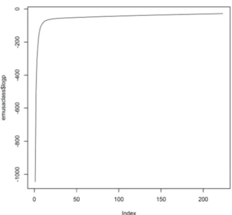
Figure 5 shows the convergence of log-likelihood. The log-likelihood increase very fast within first 20 iterations and slow after.

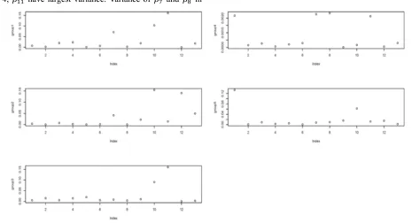
When estimating, is a vector includes ₎, … , _·) . We let M 1 and estimate of are computed from dataset directly. Log-likelihood convergence is one way to meet our goal, however, this criteria can not guarantee the stability of parameter estimates. Table 1 gives the results of estimation and Figure 3 shows the variance of parameter estimates. All variance are obtained based on 10 time computation. In group 1, 3, 4, have largest variance. Variance of _¸ and _¹ in

group 4 are large compared with other estimate. In group 4 and 5, variance of and _C are large.

Table 1. Parameter estimation with 0.9, M 1.

•º» •º¼ •º½ •º¾ •º¿

) 0.000 0.000 0.000 0.000 -0.160

C) 0.000 -0.503 0.560 -0.013 0.867

·) -0.655 0.000 1.015 -0.079 0.245

À) 0.000 0.000 -0.693 -0.002 -0.643

`) -1.037 -1.001 0.820 -0.019 0.337

Á) -0.135 -1.093 -1.310 -0.055 -0.951

¸) 0.178 0.000 -0.063 0.060 0.000

¹) -2.020 0.004 -0.030 0.039 -0.103

Â) -0.896 1.118 -1.456 0.000 -0.003

A) -0.148 0.471 -0.433 0.000 0.000

) -1.835 0.000 -0.002 0.032 0.000

C) 0.000 -0.393 0.000 0.000 -0.216

·) -0.509 0.168 -0.166 0.000 0.000

Figure 6. Variance of Estimate.

5.4. Bayesian MSVM

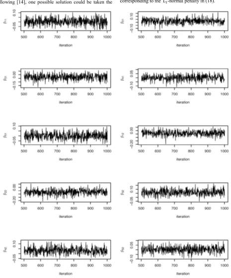
First, we test our Bayesian MSVM on a dataset , named wine, in the UCI data repository. It classifies a given silhouette as one of four types of vehicle based on 18 predictors. 500 training samples were selected and the remaining 346 samples as the testing set. All the 18 predictors were used as input variables and all the inputs are normalized to have zero mean and unit variance. We ran our MCMC algorithm for 1000 iterations and burn in 500. Figure 7 is the sample paths for the coefficients for two predictors, there is no trend among them. In fact, the sample paths of all the parameters are stationary, which indicates our MCMC is convergence. The classification error on the training set is 39% 195/500, and the

Figure 7. The sample paths for the coefficients of the first two predictors.

6. Discussion

In the Bayesian MSVM framework, we need to use the truncated multivariate normal distribution to satisfy the sum to zero constraint on f . ,i.e. ∑₎ &₎ x 0 for # 1, ⋯ , u, but it sacrifices the efficiency of the computation. In our ca

suppose

X È x xC

⋮ x

Ê , D

Ì Í Î

C ⋯

C C ⋯ C

⋮ ⋮ ⋯ ⋮

" C ⋯ "

Ï Ð Ñ

(31)

then the sum-to-zero constraint is equivalent to X ∑₎ β₎

0 . If the design matrix X is of full rank, then ∑₎ β₎ 0_" or D1 0_" can guarantee the constraint.

Following [14], one possible solution could be taken the

reparameterization procedure below

D BH (32)

where H I 1 1 . However, since the matrix H is singular, it is impossible to get the density distribution for the parameters B from the distribution of D by using the density transformation formula. One possible solution for this issue could be solved by looking for a kernel function corresponding to the -normal penalty in (18).

7. Conclusion

This paper considered the Bayesian multicategory support vector machine (MSVM). For the problem, a Bayesian framework for MSVM was developed based on stochastic variational inference and inducing points. The proposed Bayesian approach is robust against outliers with advanced accuracy and guaranteed error rate similar to the frequentist formulation of the SVM. The Bayesian method also has the advantage of modeling with high flexibility, automatic parameter tuning, and providing estimates of uncertainty in predictions. The numerical studies suggested that the proposed method has good predication accuracy and works well for practical situations.

References

[1] Boser, B. E., Guyon, I. M., & Vapnik, V. (1992). A training algorithm for optimal margin classifiers. In Fifth Annual Workshop on Computational Learning Theory, Pittsburgh, 1992.

[2] Vapnik, V. (1998). Statistical learning theory. Wiley, New York. [3] Burges, C. J. C. (1998). A tutorial on support vector machines for pattern recognition. Data Mining and Knowledge Discovery, 2(2), 121-167.

[4] Nicholas G. Polson and Steven L. Scott (2011). Data Augmentation for Support Vector Machines. Bayesian Analysis, 6, 1-24.

[5] Cortes, C., Vapnik, V. (1995) Support-Vector Networks, Machine Learning.

[6] Henao, R., Yuan, X., Carin, L. (2014) Bayesian Nonlinear

Support Vector Machines and Discriminative Factor Modeling. Neural Information Processing Systems Conference.

[7] Hoffman, M. D., Blei, D. M., Wang, C., Paisley, J. (2013) Stochastic Variational Inference. Journal of Machine Learning Research, 14, 1303-1347.

[8] Hensman, J., Fusi, N., Lawrence, N. D. (2013) Gaussian processes for big data. Conference on Uncertainty in Artificial Intellegence.

[9] Fernández-Delgado, M., Cernadas, E., Barro, S., Amorim, D. (2014) Do we need hundreds of classifiers to solve real world classification problems? Journal of Machine Learning Research, 15, 3133-3181.

[10] Mohri, M., Rostamizadeh, A., Talwalkar, A. (2012) Foundations of machine learning. MIT press.

[11] D. F. Andrews and C. L. Mallows (1974). Scale Mixtures of Normal Distributions. Journal of the Royal Statistical Society. Series B, 36, 99-102.

[12] Mike West. (1987). On Scale Mixtures of Normal Distributions. Biometrika, 74, 646-648.

[13] Yoonkyung Lee and Zhenhuan Cui (2006). Characterizing the Solution Path of Multicategory Support Vector Machines. Statistica Sinica , 16, 391-409.

[14] Zhihua Zhang and Michael I. J ordan (2006). Bayesian Multicategory Support Vector Machines Proceedings of the Twenty-Second Conference Annual Conference on Uncertainty in Artificial Intelligence , 552-559.