On the Use of q-exponential Functions for Developing Stem Profile and Volume Models

On the Use of q-exponential Functions for Developing

Stem Profile and Volume Models

Petras Rupšys

Department of Forest Management, Aleksandras Stulginskis University, Kaunas, LT-53361, Lithuania

Abstract

The National Forest Inventory in Lithuania has collected Scots pine (Pinus sylvestris) and Norway spruce (Picea abies) trees measurement data across the country. Investigations to determine the suitability of these data for updating stem profile and volume models are required. New models for stem volume and stem profile (taper) were developed using a q-exponential function in the symbolic computational language MAPLE. Work associated with the National Forest Inventory has derived very accurate Scots pine and Norway spruce trees stem profile equations that have an application not only in deriving total tree volume estimates, but as a cost-effective mensuration tool to estimate stem volume at any part of the trunk. Three previously constructed models and a new q-exponential model for stem profile and stem volume were employed to compare predicted values with empirical values of diameter outside bark and stem volume. Performance statistics for the stem volume and stem profile equations included four statistical indices: mean percentage of absolute bias, precision, Acaike’s Information Criteria, and an adjusted coefficient of determination.

Keywords

Stem Profile Model, Stem Volume Model, Q-Exponential Function

1. Introduction

Foresters have a long history of being aware of the variability in individual tree form and trying to model it so that the overall stem profile can be described more precisely. Stem profile equations are used to predict diameters at any given height, and provide a sure method to volume estimation for the different portions along the stem. Compatibility between taper and volume equations is characterized as when the total volume obtained by summation of the sections whose volumes are defined using the taper equation (or integrating the taper function) is approximately identical to the volume calculated by the volume equation. Two approaches are commonly used to describe tree form and to estimate stem volume at any part of the trunk. One expresses variable form as a single continuous function. The other expresses variable form with a step function in such a way that the bole is separated into segments by inflection points with form being constant within each segment and different between segments. Examples of the first approach are the variable-exponent stem profile models by Kozak[1-3]. In these a single continuous function with a changing exponent from ground to tip describes the neiloid, paraboloid, and several intermediate forms[2]. Example of the second approach is a segmented polynomial stem profile model by Max and

* Corresponding author:

[email protected] (Petras Rupšys) Published online at http://journal.sapub.org/ijbe

Copyright © 2012 Scientific & Academic Publishing. All Rights Reserved

Burkhart[4]. This approach uses different models for different parts of the stem, thus each can be reasonably simple. Since the joint points are usually estimated in the process of fitting the model to data, nonlinear techniques are required in parameter estimation. The majority of stem profile models investigated to date are species-specific, and all the mathematical expressions in these stem profile models are empirical equations.

Traditionally, the relationship between volume and predictor variables has been modeled based on simple nonlinear regression. Numerous equations forms have been developed to predict tree volume. Most of these volume equations have been developed by combining predictor variables diameter at breast height and total height in various ways. The logistic-like growth models provide a most powerful tool for explaining the ubiquity of sigmoidal curve in biological systems. Most generalized sigmoid curves can be described by ordinary differential equations[5]. One -parameter generalizations of the exponential and logarithmic functions have been proposed by Tsallis[6] in the context of nonextensive statistical mechanics. The Tsallis definitions of the q-exponential and q-logarithmic functions have been applied successfully to model scots pine trees growth[7].

Our main contribution is to expand stem profile and stem volume models by using q-exponential functions and to compare the taper equations’ performance in predicting the diameter outside the bark at any given height and stem volume for Scots pine and Norway spruce species.

Table 1. Summary Statistics of the Data Set for Scots Pine and Norway Spruce Trees Across Lithuania Analyzed Using 8 Models in the Present Study

Data Number _{of trees} Min Max Mean _Dev. St. Number _{of trees} Min Max Mean _Dev. St.

Estimation Validation

Scots pine

D cm) 900 3.8 58.5 26.5 9.9 1025 5.2 62.8 26.5 10.2

H (m) 900 4.1 35.2 21.8 5.1 1025 3.8 35.2 21.7 5.2

A (yr) 900 19 161 80.1 25.6 1025 21 164 80.6 26.2

Norway spruce

D cm) 500 7.8 52.4 23.6 8.6 523 7.0 49.8 23.1 8.4

H (m) 500 7.5 33.0 21.6 5.3 523 7.6 33.8 21.5 5.0

A (yr) 500 34 120 69.2 18.9 523 30 150 68.7 20.3

2.1. Data

We focus on the modeling of Scots pine (Pinus sylvestris) and Norway spruce (Picea abies) tree data sets. Scots pine and norway spruce tree stands dominate Lithuanian forests, growing on Arenosols and Podzols forest sites and covering 725500 ha, 427000 ha, respectively. Stem measurements for 1923 Scots pine trees and 1023 Norway spruce were used for stem volume and profile models’ analysis. All data were collected during 1979-2008 across the entire Lithuanian territory, except for Kuršių Nerija National Park (latitude, 53°54’ - 56°27’ N; longitude, 20°56’ - 26°51’ E; altitude, 10 - 293 m). Mean temperatures vary from -16.4℃ in winter to +22℃ in summer. Precipitation is distributed throughout the year although predominantly in summer, the average is, approximately, 680 mm a year. Temporary circle test plots were placed in each of 42 Lithuanian state forests in randomly selected clear-cutting areas. Diameter over bark and under bark of each stem in a plot was measured every 2 meters, starting from the diameter on the root collar, 1, 1.3, 3, 5, etc. All section measurements include of 24,646 data points (Scots pine trees) and 13,039 points (Norway spruce trees). Diameter was measured to an accuracy of 1 mm.

The practical situation does not permit us to have two independent data sets. Therefore, the single data set is equally utilized for model estimation and validation. A random sample of 900 Scots pine trees (total number 1923) was selected for model estimation and the remaining data set of 1023 Scots pine trees is utilized for model validation. The Norway spruce sample data set of 1023 trees was randomly divided: 500 trees for estimation and 523 for validation. Summary statistics for diameter outside bark at breast height (D), total height (H) and age (A) of all trees used for model comparison are presented in Table 1.

2.2. Stem Volume and Profile Models

For given accurate data set, to determine true stem volume is complicated problem. Smalian's equation calculates the actual (measured) volume of paraboloids and has no notable bias for upper stem sections as the tip is small. However, bias for butt section may exceed 15 percent[8]. In our analysis, we interpret the volume calculated by equation (1) as the observed volume

(

2 2

)

2 _{1 1}

1 2 1 1 3 40000 3 i i i

n _{ik ik ik ik ik}

k i

in in

d d d d L

V d L π − _{+ +} − − =  _{+ + ⋅ ⋅}      = _{ } ⋅ ₊     

∑

₍₁₎

Four alternative models (described below) were used to predict stem volume: the three-parameter Schumacher -Hall[9] model (Eq. (2)), the two-parameter Burkhart[10] model (Eq. (3)), the six-parameter linear Meyer[11] model (Eq. (4)), and the six-parameter q-exponential model (Eq. (5)) developed by Rupšys and Petrauskas[7].

3 2

1

exp( )

V₌

_β

D Hβ β

(2) 2

1 2

V=β β+ D H (3)

2 2

1 2 3 4 5 6

V=β β+ D+βD +β DH+βD H+β H (4)

(

)

(

)

(

)

6

2

1 1 4

1 3 6 5

5

1 exp 1

V _βHβ _β β _{β β} D β

β

−

+

 

= _ − − − _

  (5)

where β β1− 6 are parameters estimated from the data,

[ ]

    < ≥ =

+ _{0, 0}

, 0 , a if a if a a .

The most commonly used stem profile models were developed by Max and Burkhart[4] and Kozak[1,3]. In this study, three known stem profile models and one newly developed model were evaluated.

Sharma and Parton’s[12] variable-exponent single continuous function stem profile model was written as:

2 4 3 2 37 . 1 37 . 1 1 z z H H h H D

d β β+β +β

           − −

= (6)

where z=_Hh , d is the diameter outside bark at a given

height h, D is the diameter outside bark at breast height,

H is the total tree height from ground to tip, β β1− 4 are parameters estimated from the data.

Max and Burkhart’s[4] segmented polynomial stem profile model is written as follows:

(

)

(

)

(

) (

)

(

z

) (

I z

)

z I z z z D d − − + − − + − + − = 2 2 2 2 4 1 1 2 1 3 2 2 1 2 2 1 1 α α β α α β β

β ₍₇₎

data and

(

)









−

≥

=

−

otherwise

z

if

z

I

_{i i} i

0

,

0

1

α

α

_.

A few different formulations of stem profile models were proposed by Kozak[1-3]. In this study, one variable-exponent single continuous function stem profile model was utilised in the following form[3]

(

)

4 0.1 1

4 5 6 7 8 9

3

2 exp

1

Q

D

z _H X D H X

d

₌

_β

D H X

β β β +β − +β +β −+β +β

(8) where 1₃ 1₃ 1 1 z X p − = − , 1 3 1

Q= −z , p=1.3_H

1 9

β β− are parameters estimated from the data.

A new segmented stem profile model developed by Rupšys and Petrauskas[7] was defined in the following form using a q-exponential function and parabola

(

)

( )

(

)

(

)

(

)

             − − − ≥ − + − = ₋ + 8 2 1 1 7 8 7 6 5 1 2 4 3 1 1 exp 1 , 1 1 β β β β β β β α β β β z z if z z D

d (9)

where β β1− 8 are parameters estimated from the data. The main advantage of using stem profile curves is that, if tree profiles can be described accurately, the volume for any merchantability segment can be computed using integration. Hence, the stem profile equation of stem diameter,

(

, ,

)

d d D H h= , allows us to revise the prediction for total stem volume, V

(

D,H

)

, in the following form

(

)

(

(

)

)

2

0

, , ,

40000

H

V D H = π

∫

d D H h ⋅dh (10)

2.3. Statistical Analysis and Comparison of Model Performance

In the general formulation of the nonlinear and linear fixed-effects models (Eqs. (2)-(9)) used in this study, the error terms ei (for height, volume and taper models) are assumed to be independent and identically distributed with mean of zero and non constant variance. A power variance function was incorporated for the stem volume and taper models. Following Harvey[13], we shall refer to it as the multiplicative heteroscedastic model. The power variance function was defined as 2 2 2

i Dγ

σ =σ , where

γ

is the variance function coefficient, D is the variance covariate (diameter outside bark at breast height). The variance function coefficient γ was estimated by the modified two-step procedure proposed by Harvey[13]. Equations (2)-(9) were fitted to the observed data using weighted least-squares regression (NonlinearFit procedure and LinearFit procedure in the symbolic computational language MAPLE.

The four stem profile and volume models were compared with the observed values of the diameter outside the bark and the stem volume. Numerical and graphical analyses of the residuals were used as criteria for comparing the stem profile

equations. The performance statistics of the stem profile equations for the diameter and the volume included four fit statistics: the mean percentage of absolute bias (MPB), the precision (P), the Akaike’s Information Criteria (AIC), and an adjusted coefficient of determination (R2):

1 1 *100 n i i i n i i y y MPB y ∧ = = − =

∑

∑

1 2 2 2 1 1 1 1 1 n n

i i i i

i i

P y y y y

n n ∧ ∧ = =  _{    }  =_{ } − _ +_{ } − _ _ −      

∑

∑



ln( ) 2

AIC n RSS= + p,

2

1 n

i i i

RSS y y∧

=   = _ − _  

∑

(

)

2 2 ₁ 2 1 1 1 n i i i n i i y y n R

n p _{y y}

∧ = =  ₋    −   = − − ₋

∑

∑

where n is the total number of observations used to fit the height, stem volume and taper models, p is the number of model parameters, yi , yi

∧

, and y are the measured, estimated and average values of the dependent variable (stem volume, diameter outside bark), respectively. The AIC can generally be used for the identification of an optimum model in a class of competing models[14]. The first term on the right hand side of AIC equation is a measure of the lack-of-fit of the chosen model, while the second term measures the increased unreliability of the chosen model due to the increased number of model parameters.

3. Results and Discussion

Scots pine trees.

Table 2. Estimated Parameters of All Models Applied to the Estimation Analysis Data Set

Eq. β1 β2 β3 β4 β5 β6 β7 β8 β9

Norway spruce

(2) -10.3747 1.7188 1.3690 - - - - -

(3) 0.0213 0.00004

(4) -0.0981 0.0228 -0.0010 -0.00002 0.00006 -0.0041

(5) 0.0033 1.3841 0.9116 0.1424 -0.5465 0.9493

(6) 0.9891 0.0410 -0.1320 0.4319

(7) -0.1475 2.4420 67.0639 -2.9956

(8) 0.9226 0.9345 0.0976 0.4567 -0.4193 0.4492 1.5273 0.0223 -0.2013

(9) 1.3742 0.9709 0.4768 -1.0633 0.0557 -610.322 -0.6996 37.349

Scots pine

(2) -9.5385 1.7795 1.0200

(3) 0.0476 0.00003

(4) 0.0904 -0.0036 0.00001 0.0009 0.00002 -0.0121

(5) 0.0222 0.9920 0.3523 0.1331 -0.0833 0.7413

(6) 1.2575 -0.0607 -0.1639 0.4984

(7) -0.3222 1.5444 48.1506 -1.7529

(8) 0.9753 0.9423 0.0672 0.4293 -0.1159 0.4089 -0.3667 -0.0026 0.0088

(9) 1.4970 0.9174 1.2140 -1.5759 0.4131 -4.7894 -0.6965 12.385

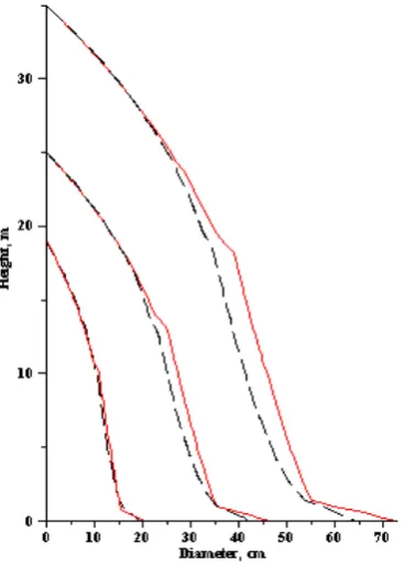
Table 3. Estimation Goodness of Fit Statistics for All Models Applied to the Estimation and Validation Analysis Data Sets

Eq. Estimation No. Obs. Validation No. Obs.

MPB P AIC 2

R MPB P AIC R2

Taper models (Norway spruce)

(6) 8.84 2.167 65745 0.958 6378 9.27 2.287 69698 0.952 6665

(7) 6.88 1.646 62215 0.976 6378 7.40 1.794 66407 0.970 6665

(8) 5.85 1.443 60572 0.981 6378 6.31 1.571 64709 0.977 6665

(9) 5.90 1.497 61028 0.980 6378 6.52 1.660 65410 0.975 6665

Volume models (Norway spruce)

(2) 7.60 0.064 372 0.982 500 8.72 0.073 550 0.975 525

(3) 8.26 0.070 465 0.978 500 9.70 0.082 668 0.969 525

(4) 7.60 0.064 372 0.982 500 8.73 0.073 550 0.975 525

(5) 7.70 0.064 371 0.982 500 8.94 0.073 560 0.975 525

(6)&(10) 8.34 0.073 504 0.977 500 9.80 0.086 723 0.966 525

(7) &(10) 8.27 0.072 481 0.978 500 9.88 0.084 690 0.968 525

(8) &(10) 7.63 0.070 431 0.980 500 8.65 0.075 557 0.975 525

(9) &(10) 8.05 0.071 457 0.979 500 9.41 0.080 633 0.971 525

Taper models (Scots pine)

(6) 7.00 1.734 120804 0.975 11554 7.01 1.742 138790 0.976 13104

(7) 6.08 1.519 117569 0.981 11554 6.10 1.531 135189 0.982 13104

(8) 5.37 1.366 115295 0.985 11554 5.46 1.394 132947 0.985 13104

(9) 5.24 1.365 115293 0.985 11554 5.31 1.391 132906 0.985 13104

Volume models (Scots pine)

(2) 6.90 0.072 1396 0.983 900 6.71 0.069 1623 0.986 1025

(3) 7.83 0.078 1541 0.980 900 7.84 0.075 1797 0.983 1025

(4) 6.94 0.071 1382 0.983 900 6.68 0.068 1603 0.986 1025

(5) 6.76 0.070 1360 0.984 900 6.42 0.067 1583 0.986 1025

(6) &(10) 7.36 0.081 1608 0.979 900 7.08 0.076 1831 0.983 1025

(7) &(10) 8.13 0.089 1786 0.974 900 7.64 0.083 2002 0.980 1025

(8) &(10) 6.93 0.073 1423 0.983 900 6.70 0.069 1639 0.985 1025

For Norway spruce trees, in terms of all fitness statistics used, the both Kozak and q-exponential segmented stem profile models (8), (9) appear similar predict diameter outside bark.

Model validation procedures in this study involved assessing models behavior with the validation data set. All goodness-of-fit statistics in the validation data set are more severe than in the estimation data set.

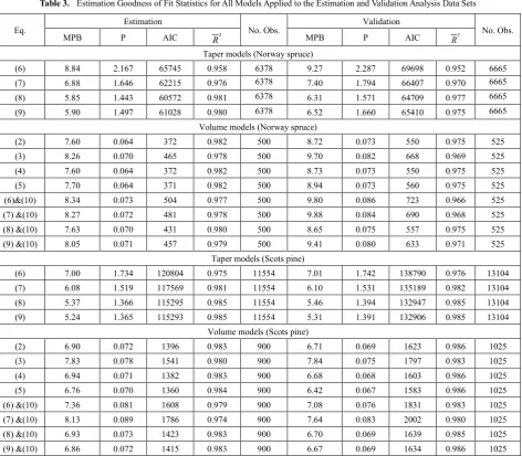
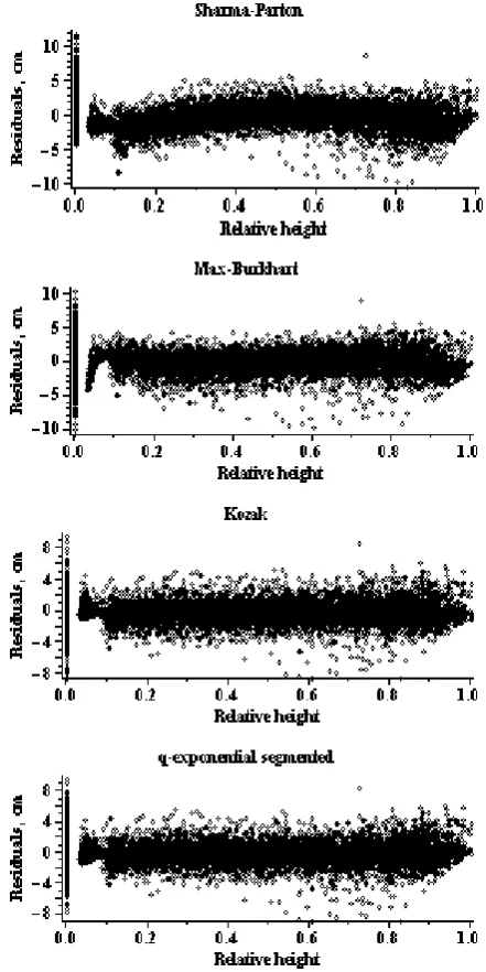
The all used models of stem profile and volume were va- lidated by the display of graphical residuals plots. Figures 1, 2, 3, 4 display residual values against predicted values (for volume models) and relative height (for stem profile models), respectively. Graphical diagnostics of the residuals for the diameter and volume predictions showed that the residuals of the q-exponential models (5), (9) had more homogeneous variance than other stem profile and volume models. These results are similar to the evaluation obtained using fit statistics (see Table 3). However, for the prediction

Figure 1. Residuals for the stem profile models (Norway spruce trees)

Figure 4. Residuals for the stem volume models (Scots pine trees) of stem volume, the residuals increased steadily with stem volume. The trend becomes less obvious when the predicted volume is less than 1.5 m3

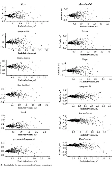
Stem profiles for three Scots pine and Norway spruce trees with the same diameter outside the bark at breast height of 15.0, 35.0 and 55.0 cm and the same total tree heights of 19.0, 25.0 and 35.0 m, respectively, using q-exponential segmented stem profile curve (Eq. (9)), are plotted in Figure 5. It is clear that all tree profiles for Norway spruce and Scots pine trees are different. A graphical examination leads to the conclusion that the difference in species is more for large trees.

Figure 5. Tree profiles for three Scots pine (dash-black line) and Norway spruce (solid-red line) trees generated using q-exponential segmented curve (9)

5. Conclusions

This study represents a systematic approach for development of stem profile models for the two conifer species across the entire Lithuanian territory. We have presented the analysis of diameter and volume estimation using the widely used stem profile equations. Overall, the q-exponential stem profile and volume equations developed here represent a significant improvement to the Honer[15], Burkhart[10] volume equations, and to the Sharma and Parton[12], Max and Burkhart[4] stem profile equations. In addition to providing an ability to estimate total stem volume, the equations can be used to estimate merchantable volume to any desired specification based on minimum top diameter or length.

The results demonstrated that for modeling the volume and diameter outside the bark, the q-exponential models (5), (9) showed the best fit for scots pine trees.

The q-exponential function presented in this study represents a general framework that can be applied to other model forms and response variables of trees.

REFERENCES

[1] A. Kozak, "A variable-exponent taper equation", Canadian Journal of Forest Research, vol. 18, pp. 1363-1368, 1988. [2] A. Kozak, "Effects of multicollinearity and autocorrelation on

the variable-exponent taper functions", Canadian Journal of Forest Research, vol. 27, pp. 619-629, 1997.

[3] A. Kozak, "My last words on taper equations", Forestry Chronicle, 80, 507-514, 2004.

[4] T.A. Max, H.E. Burkhart, "Segmented polynomial regression applied to taper equations", Forest Science, vol. 22, pp. 283-288, 1976.

[5] C. Tsallis, "What should a statistical mechanics satisfy to reflect nature?", Physica D: Nonlinear Phenomena, vol. 193, pp. 3-34, 2004.

[6] C. Tsallis, "Possible generalization of Boltzmann-Gibbs statistics", Journal of Statistical Physics, vol. 52, pp. 479-487, 1988.

[7] P. Rupšys, E. Petrauskas, "Development of q-exponential models for tree height, volume and stem profile", International Journal of the Physical Sciences, vol. 5, no. 15, pp. 2369-2378, 2010.

[8] D. Bruce, "Butt-log volume estimators", Forest Science, vol. 28, pp. 489-503, 1982.

[9] F.X. Schumacher, F.D.S. Hall, "Logarithmic expression of timber tree volume", Journal of Agricultural Research, vol. 47, pp. 719-734, 1933.

[11] H.A. Meyer, "Die rechnerischen Grundlagen der Kontrollmethode", Beiheft zu den Zeitschriften der Forstvereins, vol. 13, 122 p., 1934.

[12] M. Sharma, J. Parton, "Modeling stand density effects on taper for jack pine and black spruce plantations using dimensional analysis", Forest Science, vol. 55, pp. 268-282, 2009.

[13] A.C. Harvey, "Estimating regression models with multiplicative heteroscedasticity", Econometrica, vol. 44, pp. 461-465, 1976.

[14] H. Akaike, "A new look at the statistical model identification", IEEE Transactions on Automatic Control, vol. 19, pp. 716-723, 1974.