A DETAILED ANALYSIS OF VARIOUS DENOISING TECHNIQUES FOR CDNA MICROARRAY IMAGES

(1)

248 |

P a g e

A DETAILED ANALYSIS OF VARIOUS DENOISING

TECHNIQUES FOR CDNA MICROARRAY IMAGES

Chitra A

1

, Sunitha R

2

and Dr.H.B.Phaniraju

3

1

M.Tech student (Digital Electronics & Communication),

Rajarajeswari College of Engineering, Bangalore(India)

2

Ph.D Research Scholar and Associate Professor, Dept. of ECE,

Rajarajeswari College of Engineering, Bangalore(India)

3

Principal, Rajiv Gandhi Institute of Technology, Bangalore(India)

ABSTRACT

The image noises usually occur during the accusation or while transmission. It is necessary to remove the noise to provide further processing techniques like edge detection, segmentation, etc. In this paper the analysis is performed to remove salt and pepper noise, Gaussian noise and speckle noise using different Denoising techniques like standard median filter (MF), switched median filter (SMF), Progressive Switched Median Filter(PSMF), vector median filter (VMF), Decision Based Algorithm (DBA), Mean Filter, Weiner Filter (WF) and Wavelet based denoising using different coefficients are implemented.

The scope of the paper is to find better denoising method. The MATLAB based simulation is carried out for calculating the Mean square Error (MSE), Peak Signal to noise ratio (PSNR) and Mean Structural Similarity Index (MSSIM) values.The result obtained using Switched Median Filter and Decision Based Algorithm is performs better in removing Salt and Pepper Noise. Similarly for removing Gaussian noise and Speckle Noise by Wavelet transform.

Keywords-

Gaussian Noise, Mean Square Error (MSE), Mean Structural Similarity Index (MSSIM), Peak

Signal To Noise Ratio (PSNR), Salt And Pepper Noise And Speckle Noise

I. INTRODUCTION

The microarray image is considered to be the next generation development in bioinformatics to monitor

thousands of genes simultaneously. A microarray image is an array of spots sequences arranged in the solid surface

of glass slide. Every spots contains multiple collection of single DNA sequence [1].

During the process of experiment the mRNA of the two tissue of interest is extracted and purified, then each of

the mRNA samples are reverse transcribed into its complementary Deoxyribonucleic acid (cDNA). They are labeled

with two different fluorescent dyes which results into two fluorescence tagged cDNA (green CY3, red CY5). The

tagged cDNA are hybridized in the glass slides.

The hybridized glass slide with fluorescent dyes is scanned at different wavelength where two different images

(2)

249 |

P a g e

electronic noise, dust on the glass slide, due to laser light reflection and so on. Hence it is necessary to remove the

noise for further processing [2-6].

In this paper a detailed comparative analysis of different Denoising techniques is implemented to remove salt

and pepper noise, Gaussian noise and speckle noise.

II. TYPES OF NOISE.

2.1 Salt and Pepper Noise

The salt and pepper noise is also called as impulse noise or spike noise. A typical variety of salt and pepper

noise in a cDNA microarray image is the salt and pepper noise which will have dark pixel in bright region and bright

pixel in dark region. The white pixel (salt) and black pixel (pepper) is the kind of disturbance to the image. The

noise density can be that of the salt and pepper noise in the image. The total noise density of nd in an M×N image is

nd×M×N pixel contains noise. In general, the complete noise density of salt and pepper is d then every salt noise

therefore the pepper noise is nd/2. The salt noise and pepper noise is different noise density nd1 and nd2, therefore

the whole noise density will be:

nd = nd1 + nd2 (1)

2.2 Speckle Noise

The in cDNA microarray imaging technique speckle noise will be present so it is necessary to remove the

speckle noise. Speckle noise is considered to be multiplicative noise can be represented by the equation as below:

N(i,j)=nf(i,j)m(i,j)+a(i,j) (2)

were n(i,j) represents the noisy pixel, nf(i,j) is considered to be noise free pixel, m(i,j) is the multiplicative

noise and a(i,j) is the additive noise respectively i, j are the spatial locations. Since the effect of additive noise is

considerably small when compared with multiplicative noise (2) we can write as:

n(i,j) = nf(i j) m(i,j) (3)

Where the speckle noise intensity nf(i,j) m(i,j) is close to Gaussian noise. The logarithmic transform of

multiplicative form equation in (3) to additive noise is as:

log n(i,j) = log nf(i,j) + log m(i,j) (4)

x(i,j)=y(i,j)+n(i,j) (5)

were log n(i,j) is the noisy image in the cDNA microarray image after the logarithmic compression is denoted as

x(i,j) and the log nf(i,j) ,log m(i,j) are the noise free pixel and the noisy component after the logarithmic

compression is y(i,j) n(i,j).

2.3 Gaussian noise

Gaussian noise is an additive in nature`, and it follows Gaussian distribution where each pixel in the noisy

image is the sum of the real pixel value and random, Gaussian distributed noise value. The noise is independent of

(3)

250 |

P a g e

III. STANDARD MEDIAN FILTER

The non-linear filter is widely used to remove noise in an image than the linear filtering techniques because

linear filtering technique will tend to remove the fine details of the image [7-12]. The standard median filtering

method for the image window size taken is 3×3 where the noise and the noise free pixels are in the window. The

median value is considered in order to replace the noisy pixel to noise free pixel.

The detection of noisy pixel and noise free pixel are by considering the value of the processed pixel values

which is between maximum and minimum value with in the selected window. The dynamic range of the impulse

noise is (0, 255). When the value is of the range (0, 255) it is considered to be corrupted by the impulse noise and

the remaining pixels are the same [10].

If the dynamic range of the pixel is not between (0, 255) then it is a noisy pixel and it is replaced by the median

value or the neighborhood value of the window. By replacing the median value of each window the impulse noise is

removed. Hence we get a noise free image. Similarly the Gaussian noise and speckle noise is removed with the

standard median filter.

3.1 Algorithm for Standard Median Filter.

STEP 1: Read the noisy image I.

STEP 2: Convert the color image to gray scale image G.

STEP 3: Pad G matrix with zeros at the boundaries to get matrix P

STEP 4: Taking 3×3 matrix of pixel from matrix P.

STEP 5: Arranging the pixel in ascending order from the 3×3 matrix.

STEP 6: Calculate the median pixel and replace in matrix B.

STEP 7: Repeat step 6 for the entire image.

STEP 8: Display the denoised output image.

STEP 9: Calculate the MSE, PSNR and MSSIM value.

IV. SWITCHED MEDIAN FILTER

The switched median filter (SMF) is popularly used to remove the impulse noise. The SMF will provide better

denoising in an image [12-14]. The switched median filter it switches for the certain condition. We take the window

size to be 3×3 in the matrix. Then we calculate the maximum value in the window Wmax, the minimum value

Wmin and the median value M.

When Wmin<M && M< Wmax, if this condition satisfies then we replace the fifth value in the window if not

the condition is checked if it is satisfied then the median value is replaced or else the mean value of the window is

(4)

251 |

P a g e

4.1 Algorithm for Switched Median Filter

STEP 5: Calculate maximum pixel in the window Wmax.

STEP 6: Calculate minimum pixel in the window Wmin.

STEP 7: Calculate median in the window M.

STEP 8: Check the condition

Case A: If Wmin<M && M< Wmax put B(i,j)=0, then move to step9.

Case B: If Wmin<M && M< Wmax put B(i,j)=M, then move to step 9.

Case C: If Wmin<M && M< Wmax put B(i,j)=mean of window, then move to step9 STEP 9: Repeat step 8 for the entire image.

STEP 11: Calculate the MSE and PSNR value.

V. PROGRESSIVE SWITCHED MEDIAN FILTER

The Progressive Median Filter [15] initially the two image sequences are generated during the impulse

detection procedure. The first is a sequence of gray scale images represented as {{Xi (0)

}, {Xi

(1)_{} ,…… {X} i

(n)_{} ….},}

and binary image represented as {{Fi (0)

}, {Fi

(1)_{} ,…… {F} i

(n)_{} ….}. If F} i

(n)

=0 it is noise free, Fi (n)

=1 it is noisy. For

Xi(n-1) median value 3x3 window Mi(n-1) = Med Xj(n-1). Compute difference for Xi(n-1) and Mi(n-1) ,i.e. |Xi(n-1) -

Min(n-1)| < TD. In order to detect weather it is impulse or not the binary value of the flag should be as given in the

equation 7.1.

(6)

The threshold, TD is a pre-defined value. If Fi(n-1) < TD is noise free otherwise it is considered as noisy.

When the impulse is detected the Xi(n) is modified as in equation 7.2.

(7)

The Xi(n) =Mi (n-1)

N iteration is done or the same input pixel is replaces as Xi (n)

=Xi (n-1)

there by this

procedure the impulse detection is completed.

The second procedure is the Noise filtering the gray scale image is considered as {{Yi (0)}, {Yi (1)} ,……

{Yi(n)} ….} and binary image as {{Gi(0)}, {Gi(1)} ,…… {Gi(n)} ….} If Gi(n)=0 is noise free, Gi(n)=1 is noisy. For Yi (n-1)

(5)

252 |

P a g e

image. Replacing the value of the flag as zero and iterating to N times the noise is removed. In case if the impulse is

obtained again then the Yi (n) is modified as in equation 7.3.

(8)

The Progressive Median Filter will remove the impulse noise effectively when compared to that of the

Median Filter.

5.1 Algorithm for Progressive Switched Median Filter

STEP1: Read image I

STEP2: Convert I to gray scale G.

STEP3: Detecting image as gray scale {{Xi (0)

}, {Xi

(1)_{} ,…… {X} i

(n)_{} ….} and binary {{f} i

(0)

}, {fi

(1)_{} ,…… {f} i

(n)_{} ….}}

STEP4: The fi(n)=0 it is noise free, fi(n)=1 it is noisy.

STEP5: For Xi(n-1) median value 3x3 window mi(n-1)=med Xj(n-1).

STEP6: Compute difference of Xi(n-1) and Mi(n-1), If |Xi(n-1) - Mi(n-1)| <TD then go to step 7.

STEP8: Xi(n) =Mi(n-1) N iteration is done and stopped.

STEP7: Xi(n) =Xi(n-1) N iteration is done and stopped.

STEP9: Noise filtering of Xi(n) , generate the gray scale image as {{Yi(0)}, {Yi(1)} ,…… {Yi(n)} ….} and binary

image as {{gi (0)

}, {gi

(1)_{} ,…… {g} i

(n)_{} ….}}

STEP10: The gi(n)=0 is noise free, , gi(n)=1 is noisy.

STEP11: For Yi(n-1) median value 3x3 window mi(n-1) = Med Yj(n-1)

STEP 12: If Gi(n-1) = 1then go to step 14.

STEP 13: Yi(n) =Mi(n-1) N iteration is done and stopped.

STEP 14: Yi(n) =Yi(n-1) N iteration is done and stopped.

STEP 15: Denoised output image.

STEP 16: Calculate the MSE and PSNR value

VI. DECISION BASED ALGORITHM

Decision Based Algorithm [25], [26] here the median value itself can be noisy, especially in the case of

high noise density. It is in this case, the pixel value is replaced by the mean of the neighborhood processed pixels. In

the 3×3 window above, indicates already processed pixel values, C indicates the current pixel being processed

indicates the pixels yet to be processed. If the median value of the above window itself is noisy, then, the current

pixel value will be replaced by the mean of the neighborhood processed pixels, that is, the mean. The values of the

pixels will not be taken into account since they represent unprocessed pixels. Take the 3×3 matrix of pixels from the

padded matrix P. Calculate maximum pixel in the window Wmax. Calculate minimum pixel in the window Wmin.

(6)

253 |

P a g e

Wmin<M && M< Wmax and C=W (2, 2) replace with median value else with mean value. Repeat for all possible

3×3 matrix and replace all pixel with the median value. Thus the denoised output image is obtained.

6.1 Algorithm for Decision Based Algorithm

STEP 3: Pad the G with zeros at the boundaries to form padded matrix P.

STEP 4: Take the 3×3 matrix of pixels from the padded matrix P.

STEP 5: Calculate maximum pixel in the window Wmax.

STEP 6: Calculate minimum pixel in the window Wmin.

STEP 7: Calculate median in the window M.

STEP 8: Calculate C=W (2, 2)

STEP 9: Check the condition if Wmin<C && C< Wmax and Wmin<M && M< Wmax and C=W (2, 2) replace

With retain the same pixel value, median value else with mean value.

STEP 10: Repeat for all possible 3×3 matrix and replace all pixel with the median value.

STEP 12: Calculate the MSE and PSNR value.

VII. VECTOR MEDIAN FILTER

The vector median filter (VMF) is a nonlinear filter [16], [17], [18]. The VMF is a well-researched and widely

used due to extensive modified that can perform in conjunction with it to avoid the damage to the noise free pixel. In

the vector median filter the noisy image is taken and the 3×3 window is considered for the complete image. Every

pixel in the matrix is considered to be checked for the conditions VMF = W(i) where 1< i ≤9 in the window. ║VMF

-W║ ≤ ║Wi - W║ for 1< i ≤9. If this condition satisfies then we replace with the obtained value. The complete

image follows the same process there by the impulse noise and the speckle noise is removed.

7.1 Algorithm For Vector Median Filter

STEP 5: Considering every pixel as VMF, VMF=W(i).

STEP 6: If ║VMF -W║ ≤ ║Wi - W║ then B(i,j)=VMF.

(7)

254 |

P a g e

VIII. COMPONENT MEDIAN FILTER

The Component Median Filter [19] defined on the statistical median concept. The operation is similar to the

median filter but here the separately the median values are replaced for major colors like Red, Green and Blue. Thus

by this method we get the noise removed image for color images. This filtering method is simple in construction and

it retains the image details for the three colors. This type of filtering takes place for mainly used to remove Salt and

Pepper noise.

8.1 Algorithm for Component Median Filter

Step 1: Read the noisy image I.

Step 2: If the noisy image is color, separate each plane using MATLAB commands. Each scalar component is

treated independently.

Step 3: Pad the G with zeros at the boundaries to form padded matrix P.

Step 4: Take the 3×3 matrix of pixels from the padded matrix P.

Step 5: Then sort the pixel values within the mask in ascending order.

Step 6: For each component of each point under the mask a single median component is determined.

Step 7: These components are then combined to form a new pixel.

Step 8: Obtain the output image.

Step 9: calculate the MSE, PSNR and MSSIM.

IX. MEAN FILTER

The mean filter technique is a widely used for removing noise it effectively removes the noise while blurs the image details [10]. The mean filtering method is a linear filtering type the mean value in the window will be replaced there by the noise with high values will be removed.

9.1 Algorithm for Mean Filter

STEP 5: Calculating the mean value for the window and replace to matrix B.

(8)

255 |

P a g e

X. WIENER FILTER

Wiener filter [35], [36] is a filter used to produce an estimate of a desired or target random process by

linear time-invariant filtering an observed noisy process, assuming known stationary signal and noise spectra, and

additive noise. The Wiener filter minimizes the mean square error between the estimated random process and the

desired process .Wiener filters are characterized as the following Assumption like signal and noise are stationary

linear stochastic processes with known spectral characteristics or known autocorrelation and cross correlation

Requirement are the filter must be physically realizable/ causal.

10.1 Algorithm for Wiener Filter

STEP 3: Apply wiener filtering to the image G.

XI. WAVELET BASED DENOISING

The Discrete Wavelet Transform (DWT) [28-31] based image denoising has the following three steps. The

noisy image is considered as the input image and the two level of decomposition takes place after that the soft

thresholding [4] is applied also the wavelet coefficients are used. The reconstruction is obtained by Inverse Discrete

Wavelet Transform (IDWT). The Wavelet coefficients used are Haar, Daubechies, Symlet, Coiflet and

Biorthogonal. Using the Wavelet based noise removal the noise is effectively removed.

11.1 Algorithm for Wavelet Based Denoising

STEP 3: Perform multistage decomposition of the image G by noise using wavelet transform.

STEP 4: Apply soft thresholding to the noisy coefficients.

STEP 5: Invert the multistage decomposition to reconstruct the denoised image.

STEP 6: median filtering is applied for the reconstructed image.

STEP 11: Repeat for other wavelet coefficients.

XII. EXPERIMENTAL RESULTS & DISCUSSION

The experiment carried out in the project is to removal of the different types of the noises. The different

(9)

256 |

P a g e

20%, 30%, 40%, 50%, 60%, 70% and 80%, here noise are considered separately. The experiment shows the

comparison of performance of the linear filtering method, nonlinear filtering method and the transform technique to

remove the noise in the images which is used in the real application in the field of medical images. The Performance

parameters like MSE, PSNR and MSSIM are calculated and tabulated for the tested images.

12.1 Results for Microarray Image

Themicroarray image with Dimension 512×512 of the format JPEG (Joint Picture Expert Group) is taken

as the original image which is in color are converted to gray scale for further filtering analysis

12.1.1 Result for Filtering of Salt and Pepper Noise in Microarray Image

(a) (b) (c) (d) (e) (f)

(g) (h) (i) (j) (k) (l)

(m) (n) (o) (p)

Fig12.1: a)Original image is Microarray image in color b) Original image converted to gray scale image c)

Microarray image corrupted with 10% salt and pepper noise d) Noise removed by standard median filter e)

Noise removed by SMF f) Noise removed by PSMF g) Noise removed by VMF h) Noise removed by CMF i)

Noise removed by DBA j) Noise removed by Mean filter k) Noise removed by wiener l)Noise removed by

Wavelet thresholding using Haar coefficient m) Noise removed by DB4 n) Noise removed by Sym4 o)Noise

(10)

257 |

P a g e

Table12.1: MSE for Different Density of Salt and Pepper Noise in Microarray Image

Filter

Salt and Pepper Noise

5% 10% 20% 30% 40% 50% 60% 70% 80%

MF 32.975 34.905 37.200 40.727 44.111 52.964 61.274 75.490 93.521

SMF 11.013 11.840 14.158 17.926 21.550 26.228 29.004 31.023 29.949

PSMF 12.305 20.157 31.235 38.772 43.112 50.694 57.584 69.213 86.958

VMF 33.128 34.950 36.434 39.671 44.570 52.299 61.444 76.734 89.718

CMF 37.534 42.142 36.548 40.604 70.089 76.104 78.820 77.489 72.129

DBA 11.006 11.846 14.216 18.097 22.279 28.163 32.779 37.694 40.669

Mean 39.407 39.870 37.801 35.357 31.800 29.269 26.196 24.585 22.939

WF 36.239 39.198 37.789 35.617 31.930 29.583 26.441 24.737 23.129

Wavelet based Denoising using coefficients

Haar 48.577 45.431 37.843 32.339 27.646 25.604 22.719 21.269 19.946

DB4 46.356 43.450 35.356 29.936 25.561 23.933 21.612 20.126 19.307

Coif4 45.246 42.800 34.156 28.468 24.589 23.072 21.063 19.648 19.034

Sym4 46.701 44.272 35.734 29.869 25.735 23.813 21.650 20.179 19.314

Bior3.3 49.712 50.169 41.937 34.671 29.025 26.490 23.909 21.754 19.314

The table 12.1 the Switched Median Filter gives less value of MSE which means that the error is less for this type of

filter. Similar to the SMF the Decision Based Algorithm performs better.

Table12.2: PSNR for Different Density of Salt and Pepper Noise in Microarray Image

Filter

5% 10% 20% 30% 40% 50% 60% 70% 80%

MF 32.948 32.701 32.425 32.053 31.685 30.890 30.258 29.351 28.421

SMF 37.711 37.397 36.620 35.595 34.796 33.943 33.506 33.213 33.366

PSMF 37.229 35.086 33.184 32.245 31.784 31.081 30.527 29.728 28.737

VMF 32.928 32.696 32.515 32.731 31.640 30.045 30.246 29.280 28.602

CMF 32.386 31.835 30.925 30.201 29.674 29.316 29.164 29.238 29.546

DBA 37.714 37.394 36.602 35.554 34.651 33.634 32.974 32.368 32.038

Mean 32.175 32.124 32.355 32.646 33.106 33.466 33.948 34.224 34.524

WF 32.539 32.198 32.357 32.614 33.088 33.420 33.907 34.197 34.489

Wavelet based Denoising using coefficients as:

Haar 31.266 31.557 32.350 33.033 33.714 34.047 34.566 34.853 35.132

DB4 31.469 31.750 32.646 33.368 34.054 34.304 34.783 35.093 35.273

(11)

258 |

P a g e

Sym4 31.437 31.669 32.599 33.378 34.025 34.362 34.776 35.081 35.271

Bior3.3 31.166 31.126 31.904 32.731 33.503 33.899 34.345 34.755 35.012

The table 12.2 the Switched Median Filter, Progressive Switched Median Filter, Decision Based Algorithm

performs better.

Table12.3: MSSIM for Different Density of Salt and Pepper Noise in Microarray Image

Filter

5% 10% 20% 30% 40% 50% 60% 70% 80%

MF 0.6248 0.6265 0.6392 0.6328 0.5953 0.5174 0.4053 0.2811 0.1746

SMF 0.8809 0.8899 0.8897 0.8594 0.7966 0.7020 0.5737 0.4357 0.3170

PSMF 0.8767 0.7932 0.7056 0.6497 0.6115 0.5545 0.4633 0.3499 0.2262

VMF 0.6244 0.6279 0.6414 0.4473 0.5967 0.5108 0.4020 0.2709 0.1730

CMF 0.6110 0.6140 0.6223 0.6180 0.5831 0.5070 0.3886 0.2870 0.2181

DBA 0.8809 0.8899 0.8894 0.8571 0.7909 0.6877 0.5514 0.4038 0.2811

Mean 0.6073 0.5664 0.4800 0.4137 0.3619 0.3263 0.2969 0.2733 0.2565

WF 0.6238 0.5626 0.4662 0.4077 0.3492 0.3166 0.2888 0.2659 0.2518

Haar 0.5079 0.4976 0.4139 0.3624 0.3149 0.2926 0.2702 0.2466 0.2323

DB4 0.6246 0.6055 0.5206 0.4538 0.4162 0.3787 0.3534 0.3224 0.3080

Coif4 0.6470 0.6225 0.5414 0.4759 0.43331 0.3922 0.3632 0.3288 0.3117

Sym4 0.6144 0.5952 0.5217 0.4562 0.4199 0.3839 0.3559 0.3256 0.3081

Bior3.3 0.6456 0.6079 0.5143 0.4473 0.4089 0.3773 0.3481 0.3238 0.3030

The table 12.3 the Switched Median Filter, Progressive Switched Median Filter, Decision Based Algorithm

performs better for there are near to 1 which means that the image similarity to that of the original image is closer.

12.1.2 Result for Filtering of Gaussian Noise in Microarray Image

(12)

259 |

P a g e

(g) (h) (i) (j) (k) (l)

(m) (n) (o) (p)

Fig12.2: a)Original image Microarray image b) Original image converted to gray scale image c) Microarray

image corrupted with 10% Gaussian noise d) Noise removed by standard median filter e) Noise removed by

SMF f) Noise removed by PSMF g) Noise removed by VMF h) Noise removed by CMF i) Noise removed by

DBA j) Noise removed by Mean filter k) Noise removed by wiener l)Noise removed by Wavelet thresholding

using Haar coefficient m) Noise removed by DB4 n) Noise removed by Sym4 o)Noise removed by coif4

p)Noise removed by bior3.

Table12.4: MSE for Different Density of Gaussian Noise in Microarray Image

Filter

Gaussian Noise

5% 10% 20% 30% 40% 50% 60% 70% 80%

MF 91.102 100.39 105.50 110.86 112.41 114.51 115.66 116.29 114.46

SMF 79.118 73.403 63.951 59.156 55.180 53.837 51.973 50.266 46.924

PSMF 109.40 113.37 111.87 113.07 112.86 114.12 114.73 114.98 112.48

VMF 88.394 97.332 108.25 109.89 114.39 112.71 115.94 116.77 118.70

CMF 79.920 79.633 78.842 77.924 76.216 74.399 71.313 65.357 45.902

DBA 79.705 75.475 67.976 65.262 61.656 60.883 59.141 58.044 54.856

Mean 45.258 39.762 33.394 30.428 28.977 28.094 27.524 26.339 25.342

WF 45.358 41.011 34.698 31.409 29.832 28.796 27.920 26.991 25.751

Haar 46.285 38.754 31.704 28.194 26.277 25.442 24.913 24.230 22.578

DB4 45.599 36.905 29.471 25.732 24.275 23.600 23.227 21.833 21.055

Coif4 43.740 34.985 27.895 24.718 23.321 22.796 22.415 21.181 20.381

Sym4 45.057 36.759 29.217 25.598 24.260 23.542 23.137 21.821 21.336

(13)

260 |

P a g e

The table 12.4 the wavelet based denoising using the coefficient coiflet of order 4 gives less MSE value.

Table12.5: PSNR for Different Density of Gaussian Noise in Microarray Image

Filter

Gaussian Noise

5% 10% 20% 30% 40% 50% 60% 70% 80%

MF 28.539 28.113 27.898 27.682 27.622 27.542 27.498 27.475 27.543

SMF 29.148 29.473 30.072 30.410 30.712 30.820 30.973 31.118 31.416

PSMF 27.740 27.585 27.643 27.597 27.605 27.556 27.533 27.524 27.619

VMF 28.666 28.230 27.786 27.721 27.546 27.610 27.488 27.457 27.386

CMF 29.104 29.119 29.163 29.214 29.310 29.415 29.599 29.977 31.512

DBA 29.115 29.352 29.807 29.984 30.231 30.285 30.411 30.493 30.738

Mean 31.573 32.136 32.894 33.298 33.510 33.644 33.733 33.941 34.042

WF 31.564 32.001 32.727 33.160 33.383 33.537 33.671 33.818 34.022

Haar 31.476 32.247 33.119 33.629 33.934 34.075 34.166 34.287 34.593

DB4 31.541 32.459 33.436 34.026 34.279 34.401 34.471 34.739 34.897

Coif4 31.722 32.691 33.675 34.200 34.453 34.552 34.609 34.871 35.608

Sym4 31.593 32.477 33.474 34.048 34.281 34.412 34.487 34.742 34.839

Bior 3.3 31.343 32.191 33.033 33.473 33.810 33.952 34.167 34.329 34.491

The table 12.5 the wavelet based denoising using the coefficient coiflet of order 4 gives high PSNR value

which performs better than other filtering technique.

Table12.6: MSSIM for Different Density of Gaussian Noise in Microarray Image

Filter

Gaussian Noise

5% 10% 20% 30% 40% 50% 60% 70% 80%

MF 0.4826 0.3957 0.3191 0.2788 0.2527 0.2326 0.2219 0.2087 0.1990

SMF 0.3766 0.3108 0.2538 0.2341 0.2216 0.2144 0.2110 0.2067 0.2036

PSMF 0.2681 0.2603 0.2633 0.2526 0.2416 0.2298 0.2224 0.2116 0.2048

VMF 0.4843 0.3442 0.3185 0.2778 0.2557 0.2349 0.2205 0.2084 0.1994

CMF 0.7279 0.6771 0.5667 0.4754 0.3997 0.3324 0.2692 0.2066 0.1322

DBA 0.3732 0.3042 0.2450 0.2227 0.2039 0.2013 0.1977 0.1929 0.1890

Mean 0.5877 0.4971 0.4148 0.3725 0.3467 0.3278 0.3183 0.3108 0.3010

WF 0.5883 0.4792 0.3935 0.3537 0.3312 0.3119 0.3039 0.2978 0.2883

(14)

261 |

P a g e

DB4 0.5232 0.4913 0.4444 0.4219 0.3962 0.3789 0.3685 0.3621 0.3565

Coif4 0.5625 0.5229 0.4658 0.4397 0.4101 0.3933 0.3798 0.3729 0.3651

Sym4 0.5272 0.4948 0.4480 0.4239 0.4002 0.3846 0.3712 0.3651 0.3584

Bior3.3 0.5442 0.4990 0.4445 0.4136 0.3911 0.3763 0.3663 0.3583 0.3493

The table 12.6 the Component Median Filter performs better.

12.1.2 Result for Filtering of Speckle Noise

(a) (b) (c) (d) (e) (f)

(g) (h) (i) (j) (k) (l)

(m) (n) (o) (p)

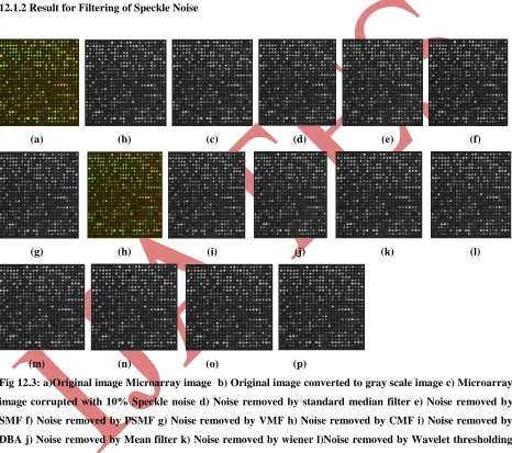
Fig 12.3: a)Original image Microarray image b) Original image converted to gray scale image c) Microarray

image corrupted with 10% Speckle noise d) Noise removed by standard median filter e) Noise removed by

SMF f) Noise removed by PSMF g) Noise removed by VMF h) Noise removed by CMF i) Noise removed by

DBA j) Noise removed by Mean filter k) Noise removed by wiener l)Noise removed by Wavelet thresholding

using Haar coefficient m) Noise removed by DB4 n) Noise removed by Sym4 o)Noise removed by coif4

(15)

262 |

P a g e

Table12.7: MSE for Different Density of Speckle Noise in Microarray Image

Filter

Speckle Noise

5% 10% 20% 30% 40% 50% 60% 70% 80%

MF 51.760 59.830 68.920 76.220 81.547 85.728 87.948 91.648 93.700

SMF 45.967 59.861 72.946 82.133 88.198 90.410 90.503 91.393 91.724

PSMF 45.300 65.645 84.936 94.476 100.30 104.28 106.22 109.43 111.05

VMF 51.728 60.119 68.565 77.349 82.490 84.066 88.718 63.530 93.511

CMF 51.400 59.404 68.157 73.108 76.338 78.447 80.588 81.906 82.812

DBA 45.979 59.886 72.938 82.097 88.164 90.351 90.455 91.266 91.516

Mean 42.053 44.802 48.461 53.475 55.604 57.987 57.285 58.320 57.748

WF 35.298 39.428 43.863 48.824 51.756 54.086 54.125 55.383 55.031

Haar 54.140 55.559 56.761 59.090 59.513 60.083 59.294 58.877 57.977

DB4 54.347 56.582 58.373 61.760 62.262 61.866 61.279 60.690 59.572

Coif4 53.068 55.829 57.995 61.158 61.675 61.623 61.029 60.133 59.085

Sym4 53.669 56.031 57.939 61.075 61.721 61.312 60.867 60.337 59.121

Bior3.3 51.839 54.594 57.633 61.047 62.749 64.200 63.037 63.530 62.249

From the table 13.7 the Weiner Filter gives less MSE value.

Table12.8: PSNR for Different Density of Speckle Noise in Microarray Image

Filter

Speckle Noise

5% 10% 20% 30% 40% 50% 60% 70% 80%

MF 30.990 30.361 29.747 29.310 29.016 28.799 28.688 28.509 28.413

SMF 31.506 30.359 29.500 28.985 28.676 28.568 28.564 28.521 28.506

PSMF 31.569 29.958 28.839 28.377 28.117 27.948 27.868 27.739 27.675

VMF 30.993 30.340 29.755 29.246 28.966 28.884 28.650 30.101 28.422

CMF 31.021 30.392 29.795 29.491 29.303 29.185 29.068 28.997 28.949

DBA 31.505 30.357 29.501 28.987 28.677 28.571 28.566 28.527 28.515

Mean 31.892 31.617 31.276 30.849 30.679 30.497 30.550 30.472 30.515

WF 32.653 32.172 31.709 31.244 30.991 30.799 30.796 30.697 30.724

Haar 30.795 30.683 30.590 30.415 30.384 30.343 30.400 30.431 30.498

DB4 30.779 30.604 30.468 30.223 30.188 30.216 30.257 30.299 30.380

Coif4 30.882 30.662 30.496 30.266 30.229 30.233 30.275 30.339 30.416

Sym4 30.833 30.646 30.501 30.272 30.226 30.255 30.286 30.325 30.413

(16)

263 |

P a g e

From the table 12.8 The Weiner Filter gives high PSNR value which performs better as filtering technique.

Table12.9: MSSIM for Different Density of Speckle Noise in Microarray Image

Filter

Speckle Noise

5% 10% 20% 30% 40% 50% 60% 70% 80%

MF 0.6923 0.6954 0.6641 0.6330 0.6036 0.5781 0.5568 0.5320 0.5142

SMF 0.8066 0.7128 0.5921 0.5162 0.4641 0.4357 0.4146 0.3973 0.3886

PSMF 0.7146 0.5891 0.4532 0.3864 0.3441 0.3214 0.3055 0.2905 0.2836

VMF 0.6909 0.6920 0.6630 0.6322 0.6016 0.5798 0.5488 0.5736 0.5145

CMF 0.6657 0.6828 0.6862 0.6781 0.6667 0.6474 0.6330 0.6204 0.6088

DBA 0.8065 0.7127 0.5920 0.5161 0.4637 0.4353 0.4142 0.3969 0.3876

Mean 0.6820 0.7047 0.7199 0.7115 0.7018 0.6878 0.6805 0.6654 0.6558

WF 0.7154 0.7310 0.7365 0.7240 0.7054 0.6894 0.6768 0.6603 0.6479

Haar 0.4440 0.4406 0.4388 0.4302 0.4312 0.4242 0.4257 0.4199 0.4259

DB4 0.5670 0.5643 0.5530 0.5465 0.5476 0.5444 0.5436 0.5350 0.5404

Coif4 0.5936 0.5949 0.5884 0.5855 0.5884 0.5822 0.5813 0.5744 0.5803

Sym4 0.5581 0.5578 0.5513 0.5474 0.5521 0.5467 0.5460 0.5390 0.5458

Bior3.3 0.5873 0.5936 0.5893 0.5838 0.5834 0.5790 0.5809 0.5736 0.5707

From the table 12.6 the Switched Median Filter performs better for there are near to 1 which means that the

image similarity to that of the original image is closer.

XIII. CONCLUSION

The scope of the paper is to retrieve the image after Denoising. The implementation was carried out using

Matlab 2011b. The Noise that was considered in the project is Salt and Pepper, Gaussian and Speckle noise. The

different filtering techniques were implemented to evaluate the performance of their noise removal in real

application images.

The image quality analysis parameters used in the project are MSE PSNR and MSSIM values. The

performance evaluation is done on the criteria that MSE value should be low and PSNR value should be high then

quality of image retrieving high, in the case of the gray scale images the value for PSNR ranges from 30 to 50 for

good performance of the image. The structural similarity of the image tested obtained after denoising which was

compared with the original image without noise. The MSSIM parameter for good quality of the image value should

(17)

264 |

P a g e

The result analysis shows that to remove the Salt and Pepper noise, the Decision based algorithm and

Switched Median Filter yields better performance. Similarly for Gaussian noise and Speckle noise the Wavelet

Transform obtained better removal noise. The MSSIM value is high for less noise density, whereas for high density

of the noises the perceptual image quality performance is poor. This paper achieves in evaluating to find the better

noise removal technique in real time applications.

13.1 Future Enhancement

This paper can further extended by implementing using different filters and it can be implemented in

hardware simulation using FPGA. Using the hardware implementation in the future may give a perfect

reconstruction using Wavelet Transform. Further implementation can be carried out for Edge detection,

Segmentation, or Pattern Recognition were for all these methods denoising is the preprocessing method. The

filtering techniques can be applied to the real application medical images.

REFERENCES

[1] M. Ki Kerr M. K, Martin M, and Churchill G. A.”, Analysis of variance for gene expression Microarray

data”, Journal of Computational Biology, vol No. 7, pp No. 819–837, 2001.

[2] Augenlicht, L. H. and Kobrin, D, “Cloning and screening of sequences expressed in a mouse colon tumor”,

Cancer Research, Vol No. 42, pp. 1088-1093, 1982.

[3] Augenlicht, L. H, Wahrman, M. Z, Halsey, H, Anderson L, Taylor J and Lipkin, “Expression of cloned

sequences in biopsies of human colonic tissue and in colonic carcinoma cells induced to differentiate in vitro

M.22”, Cancer Research, Vol No. 47, pp No. 6017-602, 1987.

[4] Schena M, Shalon D, Davis RW, Brown PO, “Quantitative monitoring of gene expression patterns with a

complementary DNA microarray”, Science, Vol No 270, pp. 467 – 470, 1995.

[5] Robert S. H, “Microarray Image Processing: Current Status and Future Directions”, IEEE Transactions Nano

bioscience, Vol No 2, pp No. 173-175, 2003.

[6] Yuk Fai Leung and Duccio Cavalieri, “Fundamentals of cDNA microarray”, Data Analysis and trends in

Genetics, Vol.19, Issue No.11, pp No. 649-659, 2003.

[7] Pawan Patidar, Manoj Gupta, Sumit Srivastava and Ashok Kumar Nagawat “Image De-noising by Various

Filters for Different Noise”, International Journal of Computer Applications, Vol No. 9, Issue No. 4, pp No.

0975 – 8887, November 2010

[8] C. Mythili and Dr. V.Kavitha, “Efficient Technique for Color Image Noise Reduction”, The Research Bullet

in of Jordan ACM , V o l . 2, January 2011.

[9] Juan Zapata and Ramon Ruiz, “On Speckle noise reduction in Medical Ultrasound Images”, Recent advances

in signals and systems, pp No. 126-131, 2009.

[10] B. Smolka, R. Lukac and K.N. Plataniotis, “Fast noise reduction in cDNA microarray images”, IEEE, 23rd

(18)

265 |

P a g e

[11] S Indu, C Ramesh, “A noise fading technique for images highly corrupted with impulse noise”, International

Conference on Computing: Theory and Applications, (ICCTA), pp. 627–632, 2007.

[12] Umesh Ghanekar “A Novel Impulse Detector for Filtering of Highly Corrupted Images “ World Academy of

Science Engineering and Technology, Vol No.14, pp No. 352-355, 2008.

[13] Pei-Eng Ng and Kai-Kuang Ma, “A switching median filter with boundary discriminative noise detection for

extremely corrupted images”, IEEE Transaction on Image Process. Vol No. 15, Issue No. 6, pp No. 1506–

1516, 2006.

[14] J Xia, J Xiong, X Xu and Q Zhang, “An efficient two-state switching median filter for the reduction of

impulse noises with different distributions”, 3rd International Congress on Image and Signal Processing

(CISP), Vol No. 2, pp.639–644, 2010.

[15] W.Zhou and D.Zhang, “Progesssive Switching median filter for the removal of impulse noise from the highly

corrupted images”, IEEE transactions on circuits and systems II. Analog and Digital Signal Processing, Vol.

46, pp.78-80, 1999.

[16] R. Lukac, “Adaptive vector median filtering”, Pattern Recognition Letters, Vol No. 24, pp No. 1889–1899,

2003.

[17] K. Manglem Singh and P. Bora. Adaptive vector median filter for removal impulses from color images.

ISCAS ’03. Proceedings of the International Symposium on Circuits and Systems, Vol No. 2, pp No. 2:II–

396–II–399, may2003

[18] V.AnjiReddy and J.Vasudevarao, “Improved vector median filter for high density impulse noise removal in

microarray images,” Global journal of computer science, online ISSN: 4172 and print ISSN:

0975-04350, Vol No. 12, Issue No. 2, pp. No 37-40, January 2012.

[19] Harish and M.R.Gowtham, “The Component Median Filter for Noise Removal in Digital Images”

International Journal of Engineering Trends and Technology (IJETT), ISSN: 2231-5381, Volume 4, Issue 5,

pp. No 1830-1836, May 2013.

[20] Anisha Bhatia, “Decision Based Median Filtering Technique To Remove Salt And Pepper Noise In Images”

Proceedings of ITR International Conference, ISBN: 978-93-82702-26-9, 18th August 2013.

[21] Windyga S. P, “Fast Impulsive Noise Removal”, IEEE transactions on image processing, Vol. 10, No. 1,

pp.173-178, 2001.

[22] Jappreet Kaur, Manpreet Kaur, Poonamdeep Kaur and Manpreet Kaur, “Comparative analysis of Image

denoising Technique”, ISSN: 2250-2459, Vol No.2, Issue No.16, pp No. 296-298, 2006.

[23] S.Kother Mohideen, Dr. S. Arumuga Perumal and Dr. M.Mohamed Sathik. “Image De-noising using Discrete

Wavelet transform”, IJCSNS International Journal of Computer Science and Network Security, Vol No .8, Issue No.1, January 2008.

[24] S. Grace Chang, Bin Yu and M. Vattereli, “Adaptive Wavelet Thresholding for Image Denoising and

Compression”, IEEE Transaction Image Processing, Vol No. 9, pp. 1532-1546, September 2000.

[25] K.S.Srinivasan, and D.Ebnezer, “A New Fast and Efficient Decision based Algorithm for Removal of High

(19)

266 |

P a g e

[26] Madhu S. Nair, K. Revathy, and Rao Tatavarti, “Removal of Salt-and Pepper Noise in Images: A New

Decision-Based Algorithm”, Proceedings of the International MultiConference of Engineers and Computer

Scientists 2008 (IMECS 2008), ISBN: 978-988-98671-8-8, Vol No.1, March, 2008.

[27] Zhou Wang, Alan C. Bovik, Hamid R. Sheikh and Eero P. Simoncelli, “Image Quality Assessment: From

Error Visibility to Structural Similarity”, IEEE Transactions On Image Processing, Vol No. 13, Issue No. 4,

April 2004.

[28] R.Alagesan, and M.A.P.Manimekalai, “An Impressive Method to Remove High Density Salt-And-Pepper

Noise from Microarray Image” International Journal of Advanced Research in Electronics and

Communication Engineering (IJARECE), ISSN: 2278-909X, vol 2, issue 3, pp. No 337-340, March 2013.

[29] Hari Om and Mantosh Biswas, “A New Image Denoising Scheme Using Soft-Thresholding”, Journal of

Signal and Information Processing, Volume.3, pp.360-363, August 2012.

[30] Akhilesh Bijalwan, Aditya Goyal and Nidhi Sethi, “Wavelet Transform Based Image Denoise Using

Threshold Approaches”, International Journal of Engineering and Advanced Technology (IJEAT), ISSN:

2249 – 8958, Volume 1, Issue 5,pp. No218-221, June 2012.

[31] Sachin D Ruikar and Dharmpal D Doye “Wavelet Based Image Denoising Technique“, International Journal

of Advanced Computer Science and Applications, Volume. 2, Issue. 3, pp. No: 49-53, March 2011.

[32] Dagao Duan and Qian Mo, “A detailed preserving filter for impulse noise removal”, computer application

and system modeling (ICCASM), print ISBN: 978-1-4244-7235-2, Volume.2, pp. No: v2-265 - v2-268,

October 2010.

[33] James Church, Dr. Yixin Chen, and Dr. Stephen Rice “A Spatial Median Filter for Noise Removal in Digital

Images” proceedings of IEEE, vol .10, pages(s) 618-623, 2008

[34] S. Md. Mansoor Roomi , T. Pandy Maheswari and V. Abhai Kumar “A Detail Preserving Filter for Impulse

Noise Detection and Removal “ ICGST-GVIP Journal, Volume 7, Issue 3, pages(s) 51-56, November 2007.

[35] Anil K. Jain,”Fundamental of Digital Image Processing”, Published by Pearson Education, 2009.

[36] Rafael C. Gonzalez, Richard E. Wood and Steven L. Eddins, “Digital Image Processing using MATLAB,

Published by Pearson Education,2005.

[37] K. P. Soman, K. I. Ramachandran and N. G. Resmi, “ Insight into Wavelets from Theory to Practice”,

Pearson Education, third edition, 2011.

[38] Smolka B, Plataniotis and K.N. Venetsanopoulos A.N, “Nonlinear techniques for color image processing”,