Efficient Learning and Inference for High-dimensional Lagrangian Systems

(1)

University of Pennsylvania

ScholarlyCommons

Publicly Accessible Penn Dissertations

Spring 4-18-2011

Efficient Learning and Inference for

High-dimensional Lagrangian Systems

Paul N. Vernaza

University of Pennsylvania, [email protected]

Follow this and additional works at:

http://repository.upenn.edu/edissertations

Part of the

Artificial Intelligence and Robotics Commons

This paper is posted at ScholarlyCommons.http://repository.upenn.edu/edissertations/301

For more information, please [email protected].

Recommended Citation

Vernaza, Paul N., "Efficient Learning and Inference for High-dimensional Lagrangian Systems" (2011).Publicly Accessible Penn Dissertations. 301.

(2)

Efficient Learning and Inference for High-dimensional Lagrangian

Systems

Abstract

Learning the nature of a physical system is a problem that presents many challenges and opportunities owing to the unique structure associated with such systems. Many physical systems of practical interest in

engineering are high-dimensional, which prohibits the application of standard learning methods to such problems. This first part of this work proposes therefore to solve learning problems associated with physical systems by identifying their low-dimensional Lagrangian structure. Algorithms are given to learn this structure in the case that it is obscured by a change of coordinates. The associated inference problem corresponds to solving a high-dimensional minimum-cost path problem, which can be solved by exploiting the symmetry of the problem. These techniques are demonstrated via an application to learning from high-dimensional human motion capture data. The second part of this work is concerned with the application of these methods to high-dimensional motion planning. Algorithms are given to learn and exploit the structure of holonomic motion planning problems effectively via spectral analysis and iterative dynamic programming, admitting solutions to problems of unprecedented dimension compared to known methods for optimal motion planning. The quality of solutions found is also demonstrated to be much superior in practice to those obtained via sampling-based planning and smoothing, in both simulated problems and experiments with a robot arm. This work therefore provides strong validation of the idea that learning low-dimensional structure is the key to future advances in this field.

Degree Type

Dissertation

Degree Name

Doctor of Philosophy (PhD)

Graduate Group

Electrical & Systems Engineering

First Advisor

Daniel D. Lee

Keywords

machine learning, robotics, motion planning, learning dynamical systems

Subject Categories

(3)

EFFICIENT LEARNING AND INFERENCE

FOR HIGH-DIMENSIONAL LAGRANGIAN SYSTEMS

Paul N. Vernaza

A DISSERTATION

in

Electrical and Systems Engineering

Presented to the Faculties of the University of Pennsylvania in Partial

Fulfillment of the Requirements for the Degree of Doctor of Philosophy

2011

Daniel D. Lee, Associate Professor Electrical and Systems Engineering

Supervisor of Dissertation

Roch Guerin, Professor Electrical and Systems Engineering

Graduate Group Chairperson

Dissertation committee

Daniel E. Koditschek, Professor Electrical and Systems Engineering

Daniel D. Lee, Associate Professor Electrical and Systems Engineering

J. Andrew Bagnell, Associate Professor Robotics Institute

Carnegie Mellon University

Maxim Likhachev, Asst. Research Prof. Robotics Institute

(4)

EFFICIENT LEARNING AND INFERENCE

FOR HIGH-DIMENSIONAL LAGRANGIAN SYSTEMS

COPYRIGHT

2011

(5)

To my parents,

(6)

Acknowledgments

I am immeasurably grateful towards my many colleagues and friends, far too numerous

to name here, to whom much of the credit is owed for making the GRASP laboratory

an interesting and intellectually stimulating place to work. I would also like to express

my gratitude towards the GRASP faculty, who have been supportive in every way of my

efforts. I credit my dissertation committee for providing indispensable guidance concerning

not only my dissertation, but also my career. I will forever be in the debt of my advisor,

Daniel D. Lee, for taking a risk hiring me as a student, for being a brilliant mentor, and

for pushing me to stay focused on my goals even when it was most difficult to do so.

I dedicate this work to my parents, Jorge and Aura, for making every sacrifice to ensure

(7)

ABSTRACT

EFFICIENT LEARNING AND INFERENCE

FOR HIGH-DIMENSIONAL LAGRANGIAN SYSTEMS

Paul N. Vernaza

Daniel D. Lee

Learning the nature of a physical system is a problem that presents many challenges

and opportunities owing to the unique structure associated with such systems. Many

physical systems of practical interest in engineering are high-dimensional, which prohibits

the application of standard learning methods to such problems. This first part of this

work proposes therefore to solve learning problems associated with physical systems by

identifying theirlow-dimensional Lagrangianstructure. Algorithms are given to learn this

structure in the case that it is obscured by a change of coordinates. The associated inference

problem corresponds to solving a high-dimensional minimum-cost path problem, which can

be solved by exploiting the symmetry of the problem. These techniques are demonstrated

via an application to learning from high-dimensional human motion capture data.

The second part of this work is concerned with the application of these methods to

high-dimensional motion planning. Algorithms are given to learn and exploit the

struc-ture of holonomic motion planning problems effectively via spectral analysis and iterative

dynamic programming, admitting solutions to problems of unprecedented dimension

com-pared to known methods for optimal motion planning. The quality of solutions found is

also demonstrated to be much superior in practice to those obtained via sampling-based

planning and smoothing, in both simulated problems and experiments with a robot arm.

This work therefore provides strong validation of the idea that learning low-dimensional

(8)

List of Figures

1.1 CMU motion capture data illustration . . . 3

1.2 Overview of learning from physical sequence data . . . 4

1.3 Trade-off between prior assumptions and dimensionality . . . 5

1.4 The PR2 robot . . . 6

2.1 A graphical model representation of a hidden Markov model . . . 14

2.2 A simple MDP . . . 19

3.1 Visualization of a kinetic Lagrangian with low-dimensional structure . . . . 30

3.2 Illustration of Snell’s law . . . 32

3.3 Interpretation of factorization provided by FCA and kinetic Lagrangians as a graphical model . . . 34

3.4 FCA applied to an inverse optics problem . . . 37

4.1 Illustration of Theorem 4.4.1 . . . 44

5.1 Graphical model associated with the GPDM . . . 47

5.2 Overview of method for sequence data modeling . . . 48

5.3 Reconstruction of novel trajectories from pairs of key frames . . . 49

5.4 Quantitative results of FCA reconstruction experiment . . . 51

5.5 A few views of an experiment reconstructing a novel action sequence . . . . 52

5.6 Robot gait reconstruction experiment . . . 53

5.7 Quantitative results from gait reconstruction experiment . . . 54

6.1 Visualized result of Bayesian estimation of non-conservative force field with predicted trajectories . . . 58

6.2 Visualized result of Bayesian estimation ofconservativeforce field with pre-dicted trajectories . . . 59

8.1 Illustration of Fermat heuristic computation . . . 71

8.2 Results of multi-robot planning experiments with deterministic planner. . . 76

8.3 Illustration of low-dimensional structure in a simple arm planning problem 77 8.4 Fermat heuristic: arm planning results . . . 80

8.5 Scaling performance of Fermat heuristic in arm planning . . . 81

(12)

9.2 Subjective comparison of different methods applied to a 36-dimensional arm

planning problem . . . 91

9.3 Quantitative evaluation of SLASHDP on arm planning problem . . . 93

9.4 Visualization of learned basis for deformable robot planning problem . . . . 95

9.5 Qualitative results of deformable robot planning with SLASHDP . . . 96

9.6 Quantitative results of deformable robot planning with SLASHDP . . . 97

10.1 Geometric interpretation of LDD . . . 101

10.2 LDD shape planning results . . . 104

10.3 LDD qualitative results . . . 106

10.4 Quantitative evaluation of LDD and various methods . . . 107

10.5 Setup ofwindows experiment . . . 108

10.6 Video stills showing inefficiencies of sampling-based planning . . . 109

10.7 Video stills comparing LDD and sampling-based planner on arm planning experiment . . . 110

10.8 Quantitative results from arm planning experiment on the PR2 robot . . . 111

(13)

Chapter 1 Introduction

This work is concerned primarily with two distinct subjects: learning the nature of a physical system, and controlling a controllable physical system. In order to make the work interesting and applicable to real-world problems, it is assumed that these systems inhabit high-dimensional state spaces.

At the broadest scope, the entirety of this work is devoted to surpassing the obstacles that arise as a result of this assumption of high dimensionality. As such, it will be helpful to begin with a brief introduction to the concept of the curse of dimensionality.

1.1 The curse of dimensionality

The phrase curse of dimensionality appears to have been coined by R. E. Bellman, the

esteemed inventor of dynamic programming. In regard to the problem of the maximization of a function, he wrote [11]:

In the first place, the effective analytic solution of a large number of even simple equations as, for example, linear equations, is a difficult affair. Lowering our sights, even a computational solution usually has a number of difficulties of both gross and subtle nature. Consequently, the determination of this max-imum is quite definitely not routine when the number of variables is large.

All this may be subsumed under the heading “the curse of dimensional-ity.” Since this is a curse which has hung over the head of the physicist and astronomer for many a year, there is no need to feel discouraged about the possibility of obtaining significant results despite it.

(14)

obtained regardless. Over half a century later, we can safely say that Bellman’s optimism was warranted. Although the curse of dimensionality visits new fields as inevitably and rapidly as ever, researchers are just as rapidly developing new tools to combat and/or avoid it.

As previously mentioned, the curse of dimensionality provides a common obstacle to the solution of the seemingly disparate problems addressed in this work. The next sections give a brief overview of these problems and how each is fundamentally affected by this curse.

1.2 Learning dynamical systems

The first problem motivating this work might be descibed broadly as learning the dynamics of a physical system: given some empirical observations of the state of a physical system at sampled times, we would like to learn a model of the system’s behavior so that we might predict its behavior in novel circumstances.

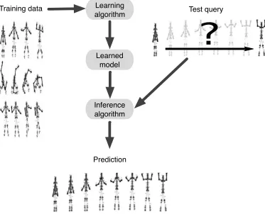
An example of this is shown in Fig. 1.2. We are given training data consisting of snapshots of a high-dimensional physical system evolving in some predictable ways—in this case, the physical system is a human being performing a variety of exercises. Observations consist of the tracked three-dimensional positions of reflective markers placed at various positions on the subject’s body, as depicted in Fig. 1.1. The concatenation of the Cartesian coordinates of all these markers comprises the state space of our system (for now, we will ignore the distinction between state and observation spaces).

We would now like to devise a learning algorithm that produces some sort of model

of the dynamics exhibited by the observations as they traverse the high-dimensional state space. The model should be such that we can subsequently perform different types of

queries about the learned dynamics by evaluating an inference algorithm that answers

queries about the learned model. The query depicted in Fig. 1.2 requests the most likely observation sequence interpolating two specific, previously-unobserved observations, cor-responding to start and end poses of a “jumping jack” motion. Evaluating the inference algorithm on this query yields a predicted sequence of high-dimensional observations, which should hopefully be similar to a jumping jack motion previously observed in the training set, while also being consistent with the boundary conditions we specified in the query.

As will be discussed in some detail later, this type of problem is most commonly analyzed from either a machine-learning or control-theoretic point of view. From the

control-theoretic perspective, this might be treated as a problem in system identification,

(15)

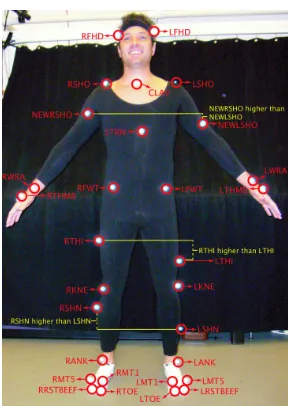
Figure 1.1: Subject wearing motion capture suit with attached retroreflective

mark-ers. (Image courtesy of the CMU Graphics Lab Motion Capture Database project,

http://mocap.cs.cmu.edu)

to the one just described, include speech recognition, stock market prediction, helicopter control, human activity recognition, and natural language processing, just to name a few. For many non-trivial applications, the basic issue is the same: as we increase the dimensionality of the problem (i.e., the number of markers in the example described), the curse of dimensionality makes it exponentially more difficult to build an accurate model and query it efficiently. From a statistical/learning-theoretic perspective, this is to say

that the sample complexity of the problem grows very rapidly with the dimension; i.e.,

unless we make some assumptions about the model, we would need an infeasible number of examples to learn it well. Moreover, from a computational efficiency perspective, many of the algorithms we would use to perform inference would also become intractable in high dimensions.

(16)

!

Training data Learning Test query

algorithm

Learned model

Prediction Inference algorithm

(17)

dimensionality

pr

ior assumptions

detailed physical modeling

black-box system identification inverse optimal control

HMM GPDM

structured Lagrangians

classic reinforcement learning

RL w/ function approx.

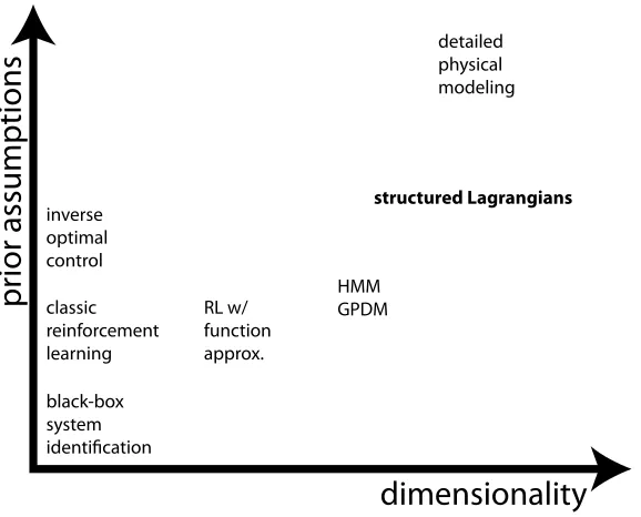
Figure 1.3: Illustration of how different learning methods trade-off prior assumptions against being able to cope with high-dimensional systems.

where the method of structured Lagrangians proposed here is compared to a variety of

other common methods for learning in dynamical systems.

1.3 Motion planning in high-dimensional spaces

The second problem motivating this work is that of how to generate motion plans for systems possessing high-dimensional configuration spaces. That is to say, we desire to find a continuous path through the system’s configuration space that connects two specified configurations subject to some constraints, such as obstacle avoidance.

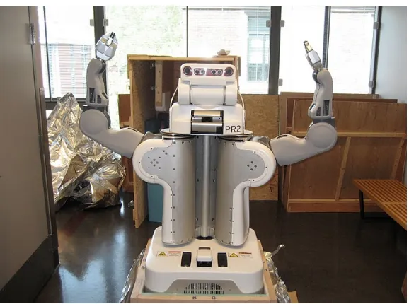
As a particular example of this, consider the robot depicted in Fig. 1.4, which is designed primarily for mobile manipulation tasks in a household environment. Many envisioned tasks for this robot require the generation of smooth, efficient paths connecting the robot’s current configuration to a desired configuration. For instance, the robot might be grasping a glass plate, and we might want it to place the plate in the dishwasher while preventing collision of the plate with the environment. We would also like it to do so as efficiently as possible.

(18)

Figure 1.4: The PR2 robot

opposed to anoptimal (i.e., efficient) one. Second, the same methods, although they work

well in relatively open environments, are likely to fail when faced with very cluttered environments.

These specific drawbacks are properties of sampling-based planning algorithms, which

are currently quite possibly the most popular methods for generating high-dimensional motion plans. There are many reasons for the success of these methods, but perhaps one of the most significant is simply that very few other methods are competitive when it comes to reliably producing plans in high-dimensional spaces.

This is somewhat distressing when one considers the simplicity of these algorithms, which basically consist of sampling random configurations, and attempting to connect them with simple paths. The random nature of sampling-based methods seems to unabashedly ignore the important underlying structure of the problem; it would therefore be surprising and unfortunate if there were no more clever method.

Obviously, this is a vast simplification that also ignores other relevant methods—proper discussion of this issue is postponed until later. However, it touches on the principal motivating factor for this work, which is the desire to find and exploit as much structure in the problem as possible. In fact, this might be thought of as a different paradigm

for developing motion planning algorithms—one that is structure-centric as opposed to

sampling-centric.

(19)

machine learning becomes relevant. Instead of using a-priori knowledge to modify the algorithm for each particular problem, it would be desirable to have the algorithm itself learn the structure of the problem and exploit it automatically. The second part of this work is devoted precisely to developing such methods.

1.4 Overview

This work is divided into two parts: the first concerned with the issue of learning from physical sequence data, and the second focusing on the problem of motion planning in high-dimensional spaces. The first part begins with a review of the literature on learning in dynamical systems in its many forms, giving a basis in which to interpret the contributions made here. We then move on to a study of how the physical nature of the systems under consideration might lead to interesting structure useful for learning and inference, proposing concrete algorithms along the way. This part concludes with an experimental study and thoughts regarding potential extensions.

After reviewing relevant literature on motion planning in high-dimensional spaces, the second part draws directly on the results generated in the first part to propose a series of novel approaches for motion planning in high-dimensional spaces. First, methods are proposed to exploit structure in such problems, assuming it is known a-priori. A method is then given to automatically learn the structure from problem data. Finally, two closely-related algorithms are given to exploit this structure—one motivated from a view of gen-erating a compressed value function for feedback motion planning, and the other based on an iterative optimization perspective. Experimental results validating these methods are given along the way.

1.5 Relation to published work

(20)

Part I

Learning structured Lagrangian

(21)

Chapter 2 Learning dynamical systems

Perhaps the best way to understand the present work in terms of current research is in terms of the general theme of learning in dynamical systems. Although there is a great body of literature falling under this general heading, much of it is sadly scattered across miscellaneous sub-domains of control theory, machine learning, and even operations research—very much to the detriment of all. This chapter makes some attempt to bring together at least a few of the major, notable, and/or relevant concepts and approaches from the different domains.

2.1 Dynamical systems

An immediate prerequisite for further discussion is a basic understanding of what a dy-namical system is and what it is about a dydy-namical system that need be learned. In abstract terms, one might define a dynamical system as an entity whose state changes in a prescribed way with the evolution of (some abstract notion of) time. An intuitive example of a dynamical system (and the primary concern of this work) is any physical system we encounter in our everyday experience. At some level of abstraction, the state of such a system could be considered equivalent to its geometric configuration and velocities, and its dynamics as those specified by Newton’s laws.

Although this physical context is the one in which we will study dynamical systems currently, a slightly broader understanding of dynamical systems will aid in understanding how this work stands in relation to current research. That said, since complete taxonomy of different categories of dynamical systems and corresponding research issues would take us too far afield, just a brief summary of a few relevant categories is now given. An example will first serve to elucidate some of these distinctions.

(22)

particles subject to forces. The state of the system can have many representations, but

for now, we represent it as the concatenated Cartesian coordinatesx of all the particles in

the system. If we consider the universe to consist only of these particles, Newton’s second

law then stipulates that there exists a function F(x,x˙) such that [7]

¨

x=F(x,x˙), (2.1.1)

where the dot notation is used to express time derivatives.

Continuous vs. discrete

This simple example already serves to illustrate a number of concepts fundamental to dynamical systems. First, the state of this physical system and the time variable upon

which it depends are both assumed to be continuousrather than discrete, since positions

and time are naturally continuous entities. More abstract physical models, by contrast, might model the state as a discrete entity.

Deterministic vs. stochastic

Newton’s Enlightenment-era model of mechanics is also prominentlydeterministic, whereas

quantum mechanics (for instance) is inherently stochastic. That is, (2.1.1) contains no

element of randomness and hence associates to each initial condition of the system, a unique trajectory; whereas a more detailed model would take into account our inherent uncertainty in our ability to predict the future state of the system.

Autonomous vs. controlled

In a similar philosophical vein, the physical system described is autonomous in that its

future state depends only on its current state, and not on any external influence. A system affected by some external influence, considered to be the effect of our own free will and

not stochasticity, might be called acontrol system.

Linear vs. nonlinear

The last distinction made here is that between linearity and nonlinearity. The forces

in Newton’s second law may be linear (i.e., springs) or nonlinear (e.g., nuclear forces) functions of the state. It is notable that this distinction only applies to systems whose state space is a vector space.

(23)

2.2 System identification

Different approaches to learning of dynamical systems may be categorized principally by the types of dynamical systems to which they apply. It should therefore come as no surprise that some of the earliest work of this nature was concerned solely with the simple linear case previously described. Although the linear assumption will prove too restrictive for the needs of the current work, it will nonetheless be useful to give an idea of the basic principles of these classical methods in order to connect the current work to well-studied issues in control theory. Moreover, the linear case given as intuition as to how to proceed in the nonlinear case, as we will see shortly.

The simplest kind of linear control system is linear in the mapping of input signals

(denoted u(t)) to output signals (denoted x(t)), where we consider these signals to form

vector spaces in the obvious way. These systems are therefore fully characterized by their behavior on a basis of input signals. This behavior takes a particularly simple form when

the system is time-invariant. In this case, we can take the input basis to be a collection

of time-shifted unit delta (or impulse) functions, and assume that the response to these

inputs are time-shifted versions of one another. The behavior of the system is thus fully

specified by theimpulse response (denoted here byh(t)); i.e., the output signal generated

by any one of the basis input signals.

For a discrete-time, scalar, causal system with a finite impulse response of length N,

the preceding discussion is summarized by noting that the state sequence can be written as the convolution of the input and impulse response:

x(t) = N−1

X

k=0

h(k)u(t−k) (2.2.1)

The goal of learning or system identification in this case would be to determine the

im-pulse response h(t) that completely characterizes this system, from observations of state

sequencesx(t) and input sequencesu(t).

The previous equation implies that for each t, we observe a single linear constraint

on the impulse response. If we stack these linear constraints in matrix form, we see that the state sequence is the multiplication of a Hankel matrix of inputs with the impulse response. By observing sufficient outputs, assuming that the inputs are varied enough, we

will eventually obtain a Hankel matrix of row rank at least N. At this point, we can solve

for the impulse response by simple linear regression. Denoting by U the Hankel matrix of

inputs, we obtain a solution via the pseudoinverse:

(24)

At this point we note that we have formulated and solved a very basic machine learning

problem as well. We definedoutput(ordependent) variablesx(t), and have modeled these

as linear functions ofinput(orindependent, orregressor) variablesu(t). Learning consists of

solving for the model parametershusing linear regression, and inference would correspond

to applying the linear model to predict future state sequences given novel inputs.

The simple model described so far can be extended in various ways. In an entirely symmetric argument, we can replace “control input” with “previous states” to obtain an autoregressive (AR) model of an autonomous system. We can then add these two models to obtain

x(t) = N−1

X

k=0

hu(k)u(t−k) + N−1

X

k=0

hx(k)x(t−k) (2.2.3)

which gives the familiar input-output representation of a linear system as the sum of a

zero-state response and azero-input response.

We can once again view the problem of identifying the impulse responses as a linear regression problem and proceed as before. From a machine learning perspective, we have now doubled our parameter set and included a new set of regressors to model the richer behavior of this more complex system.

This perspective motivates a natural extension to nonlinear systems [85]: simply replace

the regressors with nonlinear functions (orfeatures) of the original regressors. Similarly, we

need not be restricted to linear regression to estimate the output from the regressors—any conceivable regression technique could be used.

Going any further down this path brings us solidly into the realm of machine learning. That said, system identification from a control theoretic perspective is a deep subject to which this very brief treatment has not done any justice. The reader is referred to texts such as [60] for a more detailed review.

2.3 Learning latent state

We have thus far neglected the effect of the dimensionality of the state space on our ability to learn a dynamical system, since the examples of the previous section assumed a scalar state space. To gain some intuition in this area, we consider the problem of learning a

linear, autonomous system instate space representation:

(25)

Here x is now assumed to reside in a vector space of dimension N, and A is an N ×N matrix to be learned. Recalling a problem mentioned in the introduction, this is generally

a difficult problem for large N, due to a number of factors. Assuming the optimal case,

where we were to attempt to use this model to describe a system with truly linear dynamics,

our ability to determineArobustly would still depend heavily on whether we were able to

observe trajectories of a sufficiently varied nature.

In the more likely case that the modeled system were not truly linear, biaswould limit

the accuracy of such a model. We also observe the number of parameters in A grows as

the square of the dimension. Overfitting due to the large number of parameters would

therefore be a concern if we were to attempt to fit such a model in practice.

2.3.1 Hidden Markov Models

Out of these concerns and others grows the desire to leverage low-dimensional structure in dynamical systems. This basic desire forms the impetus behind what is probably the most celebrated and widespread model in machine learning for the analysis of dynamical systems: the Hidden Markov Model (HMM).

A representation of an HMM as a Bayesian network is given in Fig. 2.1. The HMM

differs from dynamical systems seen so far in a number of ways—the most salient in the

current context being that the HMM models the state (orobservation)xas being a function

of a (typically) lower-dimensional latent state. It is this latent state alone that possesses

dynamics in the HMM model. The observed state is, in this view, a marionette of sorts controlled by the latent dynamics.

In contrast to the control theoretic perspective, the HMM is usually formulated in terms of discrete latent and observation spaces, though this is not strictly necessary—a standard Kalman filter model can also be viewed as a latent space model, though in continuous space.

The HMM is also most often formulated as a stochastic model defining a joint (discrete) probability distribution over all latent states and observations. Crucially, it does so in such a way as to prevent exponential growth of the number of parameters necessary to determine the joint distribution. With no imposed structure, an arbitrary joint distribution for a

lengthT sequence with N latent states and K observation states, would entail a number

of parameters on the order of (N K)T_{. The HMM avoids this exponential growth rate by}

making two conditional independenceassumptions:

• All future states are independent of all past states, conditioned on the present state

(Markov assumption)

(26)

Figure 2.1: A graphical model representation of a hidden Markov model. Shaded areas represent unobserved states.

statext

A (typically made) additional assumption of time-invariance of the dynamics avoids even linear growth of the parameter set in the sequence length. In this case, the HMM is fully

determined by the N2 +N K parameters of the conditional probability tables P(zt|zt−1)

and P(xt|zt).

HMM inference

As previously noted, in the continuous case with linear dynamics and observation mod-els, the HMM reduces to a linear dynamical system. Inference algorithms include the

Kalman filter for forming the online state estimateP(xt|z1, . . . , zt), and the

Rauch-Tung-Streibel [76] smoother for computing the offline estimate P(xt|z1, . . . , zT).

In the discrete-state setting more often encountered in machine learning, the online

estimate is obtained via the forward algorithm, and the smoothed estimate by the

aptly-namedforward-backwardalgorithm. The latter applies dynamic programming to efficiently

compute probabilities in two passes of the data [72].

HMM learning

The problem of learning an HMM consists of determining the conditional probabilities

P(xt|xt−1) and P(zt|xt) given observation sequences x1, . . . , xT. As is so often the case,

(27)

Fascinating recent developments [23, 62, 44] have shown that it is possible to efficiently learn HMMs in Probably Approximately Correct (PAC) settings, given reasonable restric-tions; that is, with high probability, an arbitrarily-close approximation to an unknown HMM can be learned in polynomial time. In particular, [44] gives an efficient spectral algorithm for deducing the HMM from observation statistics. The key to this result is finding linear structure in this discrete problem and subsequently applying ideas from the subspace system identification literature [61, 68, 96] to obtain an analogous algorithm. This provides validation of the principle that discovering low-dimensional structure is often the key to solving high-dimensional learning problems.

Extensions

Although HMMs in the machine learning literature are typically of the discrete-state vari-ety, some work has been done to extend the HMM learning framework to continuous state spaces. As previously mentioned, the linear case is well-understood in the control systems community; hence, novel extensions typically consider the case of nonlinear dynamics and nonlinear observation functions.

A notable example [37] proceeds in a straightforward way by replacing the Kalman smoother used in a linear dynamical system with an extended Kalman smoother (EKS), a commonly-used nonlinear variant of the Kalman smoother that simply linearizes the dy-namics to obtain approximate Gaussian state distributions using the otherwise unmodified Kalman smoother. EM is then used, as in the traditional HMM, to learn the model param-eters. Though the inference step is not particularly problematic due to the use of the EKS, the maximization step requires the solution of a nonlinear maximization that is generally difficult. Cleverly, however, the nonlinear dynamics and observation functions are modeled by Gaussian radial basis functions. In this case, since the EKS provides Gaussian state distributions, it happens that the maximization step has an analytic solution obtained by solving a set of linear equations.

2.3.2 Gaussian Process Dynamical Models

Another way of extending ideas from the HMM to continuous settings comes by way of Gaussian Process Dynamical Models (GPDMs [102, 103]), which have recently been applied to the analysis of human motion capture data [103], people tracking [94], probabilistic esti-mation [50], and doubtless other problems. The GPDM can be derived from a perspective similar to the one adopted for nonlinear system identification described in Section 2.2.

Consider the following discrete-time, state-space nonlinear dynamical system model,

(28)

νt are draws of Gaussian noise:

zt = f(zt−1) +ηt (2.3.2)

xt = g(zt) +νt.

A straightforward approach to system identification for this model would be to model f

and g as weighted combinations of nonlinear basis functionsφand ψ:

f(z) = X

i

aiφi(z) (2.3.3)

g(z) = X

j

bjψj(z). (2.3.4)

φ and ψ could be chosen to represent appropriate features or regressors from which to

regress the functionsf and gby linear regression; i.e., finding weight vectorsaand bsuch

that the resulting model minimizes a squared errorloss on some training data. We could

increase the complexity of the model simply by adding more basis functions; however, adding too many basis functions would lead to overfitting.

Gaussian processes

Alternatively, we can take a statistical approach: instead of fitting a deterministic set of parameters, a prior distribution over parameters can be defined, implying a corresponding

prior distribution over functions f(z) and g(z). We would then like to use this prior

in Bayes’ theorem to produce posterior distributions over these functions given observed

training data. For example, given some training observations, z1, . . . , zT, we would want

to compute the posterior density

p(g(z)|g(z1), . . . , g(zT)) (2.3.5)

For such an expression to make sense, we must assume the existence of an underlying stochastic process; that is, for each z, there should exist a well-defined random variable

g(z) so that we can sensibly make such inferences. Fortunately, the construction of such

a process constitutes a classical result in machine learning attributed to Neal [64]. By making appropriate assumptions on the prior parameter distribution, then a central limit

argument easily shows that g(z) converges in distribution to a Gaussian in the limit as

we take the number of basis functions to infinity. The underlying stochastic process is

therefore aGaussian process (GP).

(29)

from which we can derive all of the second-order moments of the GP. Given an isotropic, zero-mean, unit-variance prior on the parameters, a straightforward computation yields,

for arbitrary z andz0,

Eg(z)g(z0) =hψ(z), ψ(z0)i. (2.3.6)

The zero-mean assumption likewise implies zero mean of the GP. Since a GP is fully determined by its first- and second-order moments, (2.3.6) gives us all the information we need to compute the inference (2.3.5). In a final twist, the basis responses are typically not even specified directly; instead, the inner product in (2.3.6) is instead defined in terms

of a positive-definitekernel function

hψ(z), ψ(z0)i:=K(z, z0), (2.3.7)

enlisting a classic machine learning trick known as the kernel trick[5].

GPDM learning and inference

With a basic understanding of Gaussian process regression, as described in the previous

section, the GPDM is fairly simple to explain. The basic concept of the method is to

use GPs to model the functions f(z) and g(z) in (2.3.3) and (2.3.4). These GPs fully

determine the joint distribution of x and z, from which any inference regarding latent

states and observations can be performed. Unfortunately, the joint distribution does not constitute a GP; therefore, Markov Chain Monte Carlo (MCMC) methods are used to perform some of these inferences.

The fact that the joint distribution is not a GP also implies that the standard GP learning technique—adapting the kernel parameters to maximize the likelihood of the data—is not strictly possible. However, this deficiency is addressed in a way borrowed from Gaussian Process Latent Variable Models [55]; i.e., the latent states are treated as deterministic parameters that are optimized to maximize the joint likelihood along with

the kernelhyperparameters.

(30)

2.4 Learning in optimal control systems

The latent state models most common in the machine learning community, such as those discussed in Section 2.3, are typically concerned with autonomous systems with no notion of control. Adding a notion of control raises a plethora of new issues that have been addressed from both machine learning and control theoretic perspectives.

Perhaps the most fundamental issue arises as a result of considering some control schemes to be superior to others. A natural question to ask in this case is what constitutes the optimal control scheme. The answer to this question is the core of what is known optimal controltheory in the control theory community. In the domain of machine learning,

such questions are typically treated in the context of reinforcement learning. A brief

summary of the latter follows first, for the sake of comparison with the learning methods just described.

2.4.1 Reinforcement learning

Reinforcement learning provides a basis in which to study problems concerning the optimal behavior of agents acting in uncertain environments. In the classical (and probably still most common) setting, the environment consists of a discrete state space, and time evolves in discrete steps.

We therefore usually envision the problem as taking place on a finite graph, such as

is illustrated in Fig. 2.2. This figure illustrates a very simple Markov Decision Process

(MDP). The dynamics of the problem are implied by the arrows, which push the agent towards a new state at each time step. Where two or more arrows emerge from a state, the agent—whose current state is illustrated by the stick-figure—is able to influence, by exerting some control action, the probability that he will transition to some particular next state over another. Upon entering each state, the agent receives a reward, illustrated

as a number of coins for each state. The agent’s goal is to find an optimal policy—i.e., a

mapping of states to control actions—to maximize his cumulative reward over time.

The state is assumed to be known in an MDP. Relaxing this assumption by adding observations and latent states yields a construct known as a Partially Observable Markov Decision Process (POMDP). The HMM might be considered a special case of a POMDP where controls are absent and the state transition graph has a certain linear structure.

Reinforcement learning typically concerns itself with two major problems: on the one

hand, the planning problem of finding an optimal policy; and on the other, the learning

(31)

Reward

Allowed transition Current state

Figure 2.2: A simple MDP

Planning

Planning for MDPs may be approached in many ways, but the most common relies on dynamic programming (DP). Central to the concept of dynamic programming is the

no-tion of a value function V(·) that gives for each state, the maximum cumulative reward

attainable starting in that state and following an optimal policy. The value function has a

simple recursive definition known asBellman’s equation[12]. Denoting byP(x0 |x0, a) the

probability of transitioning from statex to state x0 after taking action a, and denoting by

R(x) the per-state reward, Bellman’s equation is given by

V(x) := max

a

( X

x0

P(x0 |x, a)(R(x0) +γV(x0))

)

, (2.4.1)

whereγ ∈[0,1) is a given scalardiscount factor.

The optimal policy π(x) evaluated for a given state x is simply that action which

minimizes the right-hand-side of (2.4.1). Knowing the value function is therefore equivalent to knowing the optimal policy.

A classic algorithm for finding the value function consists of turning (2.4.1) into a fixed-point iteration that is guaranteed to converge to the true value function [12] and is

appropriately referred to asvalue iteration.

(32)

functions, attempting, in his words, “to trade additional computing time, which is expen-sive, for additional memory capacity, which does not exist.” [13]. This approach is usually

known today as approximate dynamic programmingor value function approximation, and

it remains a very active area of research today [30, 31, 32].

Planning in MDPs is an extremely rich and active field that, regrettably, would take us too far afield if we were to discuss it thoroughly at this point. We therefore move on to a brief summary of the learning problem.

Learning

When we speak of learning in an MDP, it usually refers to the task of planning in an MDP with unknown dynamics. Conceptually, this could be performed by first learning the dynamics (i.e., the state-transition probabilities) and subsequently using one of the planning methods described in the previous section to solve the planning problem; this is

the so-calledmodel-basedapproach. Many methods, however, are based on the observation

that the actual state-transition probabilities need not be computed explicitly if all we are concerned with is that the agent act optimally in the world; these methods are referred to asmodel-free methods.

One well-known example of such a method is Q-learning [104], which employs a

value-iteration-like fixed point algorithm to estimate a function Q(x, a) defined as the optimal

value conditioned on first taking a step with action a. Given a (potentially variable)

learning rate αt, this results in an iteration without the expectation over actions that

would require knowledge of the state-transition distribution:

Q(x, a)←Q(x, a) +αt[R(x) +γmax

a0 Q(xt+1, a 0

)−Q(x, a)]. (2.4.2)

Q-learning can be considered a special case of the more general class of temporal

dif-ferencelearning methods, which perform incremental updates based on some sort oferror

signal such as that found in the right-hand-side of (2.4.2) [97]. As with approximate dynamic programming in the known-model case, the standard approach to making such methods work in high-dimensional spaces is to use function approximation to represent

value orQfunctions [38, 91]. Perhaps the most well-known success story achieved by such

(33)

2.4.2 Inverse optimal control

Many of the ideas of reinforcement learning have equivalents in control theory under the general heading of optimal control. Whereas reinforcement learning is again usually for-mulated in terms of a discrete setting, optimal control is most often described in terms of continuous space and time. However shallow this difference may appear, it leads to fairly different solution techniques that are worth discussing briefly.

Optimal control

If there is a classical optimal control problem—just as the small-state-space MDP is the

classical reinforcement learning problem—it is most probably thelinear quadratic regulator

(LQR). The LQR is the optimal solution to the problem of controlling a linear system with a cost functional that is quadratic in the state and control signals. The LQR solution is an analytic function of the parameter matrices.

In general, the solutions to problems in continuous time and space are given by value functions that satisfy the Hamilton-Jacobi-Bellman (HJB) equation, which constitutes the continuous equivalent of the Bellman equation described previously. Unfortunately, the HJB equation is a partial differential equation that does not admit analytic solution in most cases. Discretization is therefore usually necessary to solve these problems.

Inverse optimal control

The principal philosophical difference between optimal control and reinforcement learning is that optimal control is usually concerned only with the issue of finding optimal control laws and not with any notion of learning. However, there does arise from optimal control a learning problem that is completely distinct from that of classical reinforcement learning;

namely,inverse optimal control(IOC). While reinforcement learning assumes that the cost

(or reward) functional is known but the dynamics are not, inverse optimal control makes the opposite assumption; i.e., the dynamics are known, but the cost functional is unknown. R. E. Kalman appears to have been the first to postulate and solve such a question, for the single-input LQR problem [46]. The general LQR inverse problem was ultimately solved by Boyd et. al. [15] three decades later as a simple application of linear matrix inequalities. Aside from that, it does not appear that IOC was historically a pressing issue for the control community.

In the field of operations research, aspects of what is known as inverse optimization

(34)

can be considered the solution to IOC in a deterministic MDP setting. The inverse shortest path problem is also a special case of the inverse network flow problem. Work by Ahuja and Orlin establishes dualities between different types of network flow problems and their inverse problems [4]. It should also be noted that all such problems are ill-posed as stated; the solution to this issue is usually to optimize a criterion such as minimum distance from an initial solution.

The last 10 years have marked the beginning of earnest interest in the IOC problem by the machine learning community, largely sparked by the work by Ng et. al., who referred

to the problem asinverse reinforcement learning[66, 2], and notably applied their methods

to autonomous, aerobatic helicopter flight, among other problems [65].

Closely related to IOC are methods based on astructured learningconcept. Exemplary

(35)

Chapter 3 Learning structured Lagrangians

The main objective of this work is to introduce a new category of dynamical-system-learning problems along with dynamical-system-learning and inference algorithms to solve (special cases of) it efficiently. As mentioned in the introduction, this first part of the current work describes these algorithms from a machine learning perspective. The applications of these methods to contexts of pure planning and control will be described later in the second part of this work.

What differentiates the current work from the types of approaches studied in Chapter 2

is the desire not only to learn systems of a physicalnature, but also to exploit whatever

structure we may gain from the assumption of physicality. This philosophy stems partially from a tacit admission that the possibly once hoped-for goal of a universal reasoning and learning machine, is at the very least, not within the grasp of any technology now available or even on the horizon. In artificial intelligence, the term Good Old Fashioned AI (GOFAI) is sometimes used to refer to what is now regarded as this sort of outmoded mentality [41].

The success of HMMs and other latent-state representations, in addition to the recent emergence of structured learning techniques, plainly demonstrate the advantages of ex-ploiting structure where ever possible. On the other hand, there is certainly a trade-off

to be made, since the very raison d’ˆetrefor machine learning is arguably to avoid having

to manually build every slight detail about the world into our machines. Managing this trade-off is therefore more of an art than a science—and, though one can always hope to the contrary, it is seems unlikely that this will change in the foreseeable future.

(36)

Moving on from these generalities, the immediate concern will be to elucidate the La-grangian structurewhose exploitation is hereby proposed. Before this can be accomplished, an extremely brief introduction to Lagrangian dynamics is necessary for the sake of being reasonably self-contained. The ultimate goal of this chapter will be to give a concrete, effi-cient algorithm for discovering said structure and showing how it can be exploited to learn Lagrangian systems. The next chapter will then focus on exploiting Lagrangian structure in the inference problem.

3.1 Lagrangian mechanics

We examine in this section the behavior of a physical system consisting of a collection of particles obeying Newton’s laws. We eschew this view, however, in favor of the equivalent formulation of Lagrangian mechanics. The Lagrangian view may be derived by expressing

Newton’s second law (F =ma) in a peculiar way. Specifically, we posit the existence of a

functionL(x,x, t˙ ) (wherex∈_RN_{) such that}

F = ∂L

∂x (3.1.1)

and

ma= d

dt ∂L

∂x˙ (3.1.2)

Given such a function, Newton’s second law can obviously be written as

d dt

∂L ∂x˙ −

∂L

∂x = 0. (3.1.3)

Curiously, it can be shown that a path x(t) satisfying (3.1.3) (i.e., Newton’s second law)

is also a locally extremal path of the cost functional (or action)

J{x}=

Z t1 t0

L(x,x, t˙ )dt (3.1.4)

subject tox(t0) =x0 andx(t1) =x1, for constantst0, t1, x0, x1. This is to say that local

perturbations (orvariations) ofx(t) yield no change in the cost functional—x(t) is in this

sense a local minimum or maximum of the cost functional. This is the key trick of the Lagrangian formalism: to view physical paths as those that locally optimize the action.

The importance of this view lies in the subtle but crucial observation that, as with any optimization problem, we can choose any coordinates we like in order to find a path that optimizes the action. From this we deduce that any path satisfying Newton’s laws in

(37)

Euler-Lagrange equations: ∂L ∂q − d dt ∂L

∂q˙ = 0 (3.1.5)

Therefore, in order to express the dynamics in terms of q coordinates, we need only

to find an expression for L in q coordinates, and apply (3.1.5). This can be achieved by

identifyingL as the coordinate-invariant quantity

L=T−V (3.1.6)

whereT is the potential energy of the system and T is its kinetic energy.

To summarize some key points, the Lagrangian perspective gives us an optimization-based view of physical trajectories. This view allows us easily to determine the ODEs governing these trajectories in arbitrary coordinates simply by writing down the Lagrangian and solving the associated Euler-Lagrange equations.

3.1.1 Conservation laws and Noether’s theorem

A further benefit of the Lagrangian perspective is that it leads to a deeper understanding

of how conservation laws arise in nature. A conservation law is simply a property of a

physical system that is invariant with respect to time. For example, if the total energy of a system does not change in time, then that system satisfies conservation of energy. Similarly, a physical body whose momentum remains constant in time is said to obey the law of conservation of momentum.

A classic and celebrated result due to Emmy Noether identifies precisely how such

conservation laws arise via the Lagrangian formalism. Informally,Noether’s theoremstates

that everydifferentiable symmetryof the Lagrangian leads to a corresponding conservation

law [7]. In fact, Noether’s theorem goes as far as to give a precise expression for the conservation law in terms of the symmetry. However, as the symmetries considered in this work are simple enough that a general formula is not necessary, we will not discuss this formula in further detail.

To give a concrete example of Noether’s theorem, consider a Lagrangian L(x,x˙) for

x∈RN such that ∂L/∂xi = 0, for some i. Writing the Euler-Lagrange equations for this

coordinate yields ∂L ∂xi − d dt ∂L ∂xi˙ =−

d dt

∂L ∂xi˙ = 0.

Since the time derivative of ∂L/∂xi˙ = 0, we therefore have that

(38)

for some trajectory-dependent constant k, for all time.

Making this problem even more concrete, suppose that x is the position of a particle

of massmnear the Earth’s surface, andx3 is the height of the particle above an arbitrary

reference point. Further suppose that the particle is moving freely through space, affected by no other force than gravity. The Lagrangian for this particle is given by

L(x,x˙) = m

2kxk˙

2₋_gx

3. (3.1.7)

Note that∂L/∂x1 =∂L/∂x2= 0. Therefore, by the above argument, we can deduce that

conservation laws hold for the x1 and x2 coordinates:

∂L ∂x˙1

=mx˙1 =k1 (3.1.8)

∂L ∂x˙2

=mx˙2=k2. (3.1.9)

These conservation laws constitute the familiar conservation of momentum laws in the

directions x1 andx2 parallel to the Earth’s surface.

As any student of high-school physics is aware, these conservation laws greatly simplify the analysis of simple ballistic trajectories—solving any such problem reduces to the solving

the one-dimensional ODE ¨x3 =−g, since the other velocities remain constant. Fortunately,

this phenomenon is general: the presence of conservation laws always simplifies the analysis of physical systems. Since Noether’s theorem essentially tells us that we can obtain a conservation law for free with every symmetry that we can find in our system, finding these symmetries is of utmost importance when we are faced with the analysis of any physical system. The importance of this statement cannot be stressed enough, as it may very well be considered the foundation of this entire work.

3.2 Structured Lagrangians

The method proposed here, at a high level, is simply to propose that observed trajectory data obeys a Lagrangian model and to subsequently fit the Lagrangian model from the observations. The Lagrangian model will then give a complete description of the physical dynamics underlying the trajectories, which we can consult, in principle, to answer any query regarding the behavior of the system in novel situations.

Unfortunately, we cannot hope to accomplish this in the general case, due to problems

that arise in both learning and inference. For a system ofN particles in a three-dimensional

space, the Lagrangian (written in Cartesian coordinates) is a mapL(x,x, t˙ ) :R3N×R3N×

(39)

the difference of kinetic and potential energy for the system in that state. Learning such a map in a supervised sense would therefore require training examples pairing states and differences of potential and kinetic energies—data that would most likely not be readily available in most cases.

Many physical systems of interest are also high-dimensional. Suppose we would like

again to study a system ofN particles, whereN is large. Assuming we can obtain training

data to fit the Lagrangian, we are still affected by the curse of dimensionality: a

look-up-table representation of Lwould contain a number of elements scaling exponentially in N,

thus necessitating strong prior assumptions on L in order to be able to fit it. Using the

wrong prior assumptions would lead to a biased model of L, thus limiting the ability of

such a model to fit the data well.

The problem of inference for a Lagrangian system is at least well-defined: the physical trajectories associated with a Lagrangian system are exactly those that locally optimize the action. In principle, given some representation of a Lagrangian, we could therefore find paths by solving optimization problems. However, in a high-dimensional space, finding

such local optima may prove very difficult. Each dimension of the sought-after path,xi(t)

is a function, or alternatively, a vector in an infinite-dimensional vector space. Thus, we are faced with the problem of optimization in a “high-dimensional, infinite-dimensional”

space. Such a problem might be approached using afunctional gradient descent technique,

but this entails discretization with concomitant numerical issues. Even assuming that we are able to overcome this problem, it is unclear as to whether the found optimum, of which there may be many, would be representative in any way—possibly necessitating the use of sampling to find other optima, which may prove intractable.

All of these obstacles point decidedly towards the conclusion that fitting a general Lagrangian model is neither a tractable or well-defined problem. Our aptly-named solution

to this issue is the introduction of the notion of astructured Lagrangian—a name intended

perhaps to evoke connections to structured learning. This section gradually introduces a particular kind of structured Lagrangian, though it is not the only conceivable kind. Still, arguments will be made as to why this is a sensible model for a variety of cases.

3.2.1 Conservation of energy

(40)

A simple first simplification is therefore to remove the explicit dependence of the La-grangian on time. It can be shown by Noether’s theorem that this assumption, remarkably, implies conservation of energy. On the one hand, energy conservation may seem to consti-tute a rather onerous assumption, since it would preclude modeling desirable effects such as friction and inelastic collisions. On the other hand, allowing arbitrary dissipative and external forces into our model would be unwise—a system obeying Newton’s laws sub-ject to unrestricted external forces can simulate the behavior of any kind of second-order dynamical system, which is exactly contrary to our objective of exploiting some kind of additional structure present in physical systems. In this light, ignoring dissipative effects would seem advantageous.

3.2.2 Kinetic Lagrangians

The other major assumption to be made will address most of the problems previously mentioned with the Lagrangian learning concept in one fell swoop. Namely, we will assume

the following concrete form of the Lagrangian in terms of some coordinatesx:

L(x,x˙) = 1

2m(x)kxk˙

2 _(3.2.1)

Such Lagrangians will be referred to askinetic Lagrangians in this work, as they represent

Lagrangians that possess only a kinetic energy term, and no potential energy. This kinetic energy is exactly the kinetic energy of a system of particles in Cartesian space with a common mass dependent on the position of all the particles. Though this may appear to be an odd model at the outset, kinetic Lagrangians possess a number of interesting properties that make them a suitable model for learning applications.

Supervised training

First, the conservation of energy resulting from the time-independence of this Lagrangian implies that the kinetic energy of the system within trajectories is constant, since the

potential energy is zero. Writing this energy asE, this implies that

m(x) = 2E

kxk˙ 2 (3.2.2)

Note that the Lagrangian is completely determined by the function m(x), implying that

training examples of pairs (x, m(x)) are all that we need in order to fit the Lagrangian.

m(x) is in turn determined by the inverse speed of the trajectory and a per-trajectory

constant energy. Assuming for now that we can obtain samples of trajectories in these

(41)

energy E may not be known, it represents only one unknown parameter per trajectory, which might be estimated by a method such as Expectation Maximization. If we assume

we are observing only one continuous trajectory, E is irrelevant in the sense that it only

scales our estimate of the Lagrangian by a constant factor. This constant factor becomes irrelevant when we perform inference by optimizing the Lagrangian.

Conservation laws

The other problems anticipated with the learning Lagrangian approach arose principally in the case of high-dimensional systems, the main challenge being to identify the correct prior assumption to make as to the structure of the Lagrangian in order to avoid complications owing to the curse of dimensionality. Inspired by Noether’s theorem, our approach will be to assume the presence of symmetries of the Lagrangian, which will generate conservation laws that should simplify the task of learning the Lagrangian.

Armed with a concrete form of the Lagrangian (i.e., the kinetic Lagrangian), this is straightforward. From the machine-learning perspective, a natural symmetry to propose

is a simple translational symmetry equivalent to the presence of linear low-dimensional

structure. That is, we can propose the symmetry

L(x,x˙) =L(x+sv,x˙), ∀s (3.2.3)

for a particular vector v. Owing to the form of the kinetic Lagrangian, this is equivalent

to stating that

m(x) =m(x+sv), ∀s. (3.2.4)

This is illustrated in Fig. 3.1. We say informally that m has low-dimensional structure

in the sense that m does not vary across the subspace spanned by v. Therefore, if we

wish to estimate m in the sense of supervised learning, every such symmetry reduces the

dimensionality of our estimation problem by one.

That said, it would be undesirable and physically unjustified to declare such symmetries by fiat merely because doing so simplifies the estimation problem. Instead, these presence of these symmetries will be detected by identification of the conservation laws that necessarily follow.

Accordingly, the form of these conservation laws is now derived. Suppose v above is

such that

∂m ∂xi

(x) = 0, ∀x;

that is, m does not depend on the coordinate xi. Such a coordinate will be referred to as

(42)

m(x)

v

Figure 3.1: Visualization of a kinetic Lagrangian with low-dimensional structure

imply

∂L

∂xi −

d dt

∂L

∂xi˙ = 0 1

2kxk˙

2∂m

∂x −

d

dt[m(x) ˙xi] = 0

m(x) ˙xi = k0, (3.2.5)

where k0 is a trajectory-dependent constant. We can combine this new conservation law

with conservation of energy (3.2.2) to obtain

˙ xi kxk˙ 2 =

k0

2E. (3.2.6)

Finally, observing that bothk0 andE are trajectory-dependent constants, we can combine

them into a new constantk, yielding

˙ xi

kxk˙ 2 =k. (3.2.7)

(43)

3.2.3 Geometric interpretation

Kinetic Lagrangians have an important geometric interpretation that warrants further attention here. This geometric connection may be established using a well-known corre-spondence that provides useful insight in the current context.

First, we introduce the notion of the length L of a curve x(t) on a manifold with

Riemannian metricg, which is given by

L(x) =

Z t1 t0

 

X

ij

gij(x) ˙xix˙j

 

1/2

dt. (3.2.8)

By introducing a time-reparameterized path z(t) = x(s(t)), with s(t0) = t0, s(t1) = t1,

and ds/dt 6= 0; and performing a change of variables in the expression above to s, it

is easily shown that z and x have the same length; that is, L is invariant under

time-reparameterization of curves. This coincides well with our intuition about the length of a curve, which is a geometric property independent of however we happened to parameterize

the curve. Taking gij(x) =δijm(x) yields the familiar-looking expression

Z t1 t0

p

m(x)kxkdt.˙ (3.2.9)

This can be related to the kinetic Lagrangian by applying the Cauchy-Schwarz

inequal-ity to the inner product of the functionsp

m(x)kxk˙ and 1, yielding

Z t1 t0

m(x)kxk˙ 2dt

Z t1 t0

dt≥

Z t1 t0

p

m(x)kxkdt˙

2

(3.2.10)

with equality iff. pm(x)kxk ∝˙ 1—which incidentally recovers conservation of energy

for minimizers of the Lagrangian. From this we can deduce that minimal-length curves

are also minimizers of the energy functional (i.e., the kinetic Lagrangian), up to a

time-reparameterization.

Thus, the trajectories associated with kinetic Lagrangians have a geometric

interpre-tation as geodesics of a Riemannian manifold with an isotropic metric m(x)δij.

These geodesics furthermore coincide with the intuitive notion ofshortestor

(44)

Figure 3.2: Illustration of Snell’s law

3.2.4 Fermat’s principle of least time

A further important interpretation of kinetic Lagrangian systems comes from optics. Fer-mat’s principle of least time states that the path taken by a ray of light is that which minimizes the total time needed for the ray to travel between endpoints. Taking the afore-mentioned view of kinetic Lagrangian trajectories as being minimum-cost paths, we can

identify cost with inverse speed or index of refraction to conclude that these trajectories

are also minimum-time trajectories. Therefore, we can think of these trajectories as those that rays of light would travel—possibly in a space of dimension greater than three.

Perhaps the most famous formula of optics is Snell’s law, illustrated in Fig. 3.2. When

a ray of light passes from a material with index of refraction n1 to another with index

of refraction n2, the angle of the ray made with the normal to the interface changes

according to n1sinθ1 = n2sinθ2. This can be derived from the conservation law (3.2.7)

via the identifications

n = 1

kxk˙ (3.2.11)

˙

x2 =

sinθ

n , (3.2.12)

assuming that the interface is orthogonal to the x2 coordinate direction. This reveals

that nsinθ=k, for some constant k, for all time; which implies thatn1sinθ1 =n2sinθ2.

Efficient Learning and Inference for High-dimensional Lagrangian Systems

University of Pennsylvania

ScholarlyCommons

Publicly Accessible Penn Dissertations

Spring 4-18-2011

Efficient Learning and Inference for

High-dimensional Lagrangian Systems

Paul N. Vernaza

Follow this and additional works at:

http://repository.upenn.edu/edissertations

Part of the

Artificial Intelligence and Robotics Commons

Recommended Citation

Efficient Learning and Inference for High-dimensional Lagrangian

Systems

EFFICIENT LEARNING AND INFERENCE

FOR HIGH-DIMENSIONAL LAGRANGIAN SYSTEMS

Paul N. Vernaza

Electrical and Systems Engineering

EFFICIENT LEARNING AND INFERENCE

FOR HIGH-DIMENSIONAL LAGRANGIAN SYSTEMS

COPYRIGHT

2011

Acknowledgments

Contents

List of Figures

Chapter 1

Introduction

1.1

The curse of dimensionality

1.2

Learning dynamical systems

!

dimensionality

pr

ior assumptions

1.3

Motion planning in high-dimensional spaces

1.4

Overview

1.5

Relation to published work

Part I

Learning structured Lagrangian

Chapter 2

Learning dynamical systems

2.1

Dynamical systems

2.2

System identification

2.3

Learning latent state

2.4

Learning in optimal control systems

Chapter 3

Learning structured Lagrangians

3.1

Lagrangian mechanics

3.2

Structured Lagrangians

m(x)

v