www.astrophys-space-sci-trans.net/6/9/2010/ © Author(s) 2010. This work is distributed under
the Creative Commons Attribution 3.0 License. Astrophysics and Space Sciences
Transactions
On the definition and calculation of a generalised McIlwain
parameter
J. Pilchowski1, A. Kopp2, K. Herbst2, and B. Heber2
1Geophysical Institute, 903 Koyukuk Drive, Univ. of Alaska, Fairbanks, AK 99775-7320, USA
2Inst. f¨ur Experimentelle und Angewandte Physik, Christian-Albrechts-Univ. zu Kiel, Leibnizstraße 11, 24118 Kiel, Germany Received: 3 December 2009 – Revised: 3 February 2010 – Accepted: 10 February 2010 – Published: 22 April 2010
Abstract. The L parameter, which indicates the distance where a magnetic field line crosses the equatorial plane, is defined only for an aligned magnetic dipole field. For a re-alistic planetary magnetic field, however, neither a definition nor a method to calculate this parameter are available so far. We therefore extent the definition of the McIlwain parameter for an arbitrary planetary magnetic field and numerically cal-culate it for the actual geomagnetic field. In order to do so, we first calculate the Earth’s magnetic field for 2008 with the IGRF model. To motivate a proper definition for a general
Lparameter, each component of this field will be illustrated and discussed. In a second step, we present four possible definitions for theLparameter and discuss their properties and differences with respect to the question in how far they reflect the field geometry. We contrast our method with the traditional derivation of theLparameter employing numeri-cal simulations of the cut-off rigidities of energetic particles and an empirical relation between the latter and L.
1 Introduction and basic facts
Already in the middle of the nineteenth century, Carl Friedrich Gauss demonstrated that the Earth’s magnetic field B can be derived from the sum of contributions resulting from external and internal source regions. If electric currents j can be neglected within the region of interest, i.e.
∇ ×B=µ0j=0, (1)
whereµ0is the permeability of vacuum, B can be written as the gradient of a scalar potential0, (e.g Gauss, 1836):
B= −∇0. (2)
Correspondence to: J. Pilchowski
Because of the divergence-free condition for B,0has to be the solution of the Laplace equation
10=0. (3)
In general, the scalar potential0can be expanded into a se-ries of spherical harmonics. Using spherical coordinates (r,
ϑ,ϕ), this expansion reads (e.g. Connerney, 1993):
0(r,ϑ,ϕ)=
r0
∞
X
n=1 (
r r0
n
Tn(ext)(ϑ,ϕ)+ r0
r n+1
Tn(int)(ϑ,ϕ) )
(4)
withr0representing the Earth’s radius (r0=6371 km), while Tn(ext)(ϑ,ϕ)andTn(int)(ϑ,ϕ)denote the external and internal
contributions of source regions, respectively, which can be written as
Tn(ext)(ϑ,ϕ)=
n X
m=0 (
Pnm(cosϑ ) Gmncos(mϕ)+Hnmsin(mϕ) )
, (5)
Tn(int)(ϑ,ϕ)=
n X
m=0 (
Pnm(cosϑ ) gnmcos(mϕ)+hmnsin(mϕ) )
. (6)
Gmn, Hnm, as well as gnm and hmn are the (Schmidt-)coefficients, and Pnm are the Schmidt-Legendre functions of ordersnandm. They are defined as:
Pnm(x)=Nnm p
(1−x)md mPn(x)
dxm (7)
with Nnm and Pn being the normalisation factors and the Legendre polynomials of ordern, respectively:
Nnm= (
1 m=0
q 2(n−m)!
(n+m)! m6=0
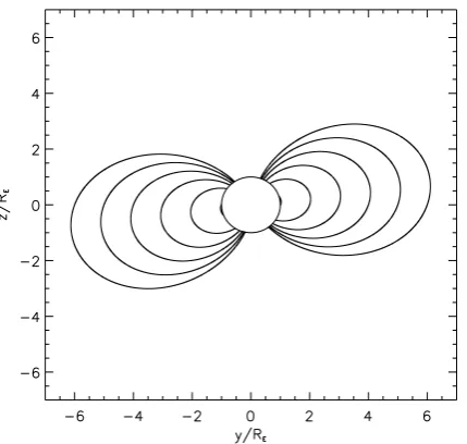
Fig. 1. Field lines of the Earth’s magnetic field calculated with the IGRF model for 2008 in cartesian coordinates with z being parallel to the magnetic field axis.
Pn(x)=
1 2nn!
dn(x2−1)n
dxn . (9)
A first approximation of the Earth’s magnetic field is a tilted dipole field, where the position of the dipole centre and the position of Earth’s centre coincide (geocentric dipole ap-proximation). This approximation is useful in regions, where the influence of the Solar wind can be neglected (cf. Sect. 2) or for the academic case in which the field is viewed from larger distances in absence of the Solar wind. At a given po-sition r, this field can be written as
B(r)=3(m·r)
r5 r− m
r3, (10)
where m1 is the magnetic moment and r=|r|. This pression simply results from the lowest-order term of ex-pansion (4), i.e.n=1 andm=0, considering only internal sources, leading to
0(r,ϑ,ϕ)=r03
g11 h11 g01
· 1 r3 x y z = m·r
r3 . (11)
Considering m to be tilted by the angle2with respect to the axis of rotation (the z-axis) and by the angle8around it, the magnetic moment can be expressed as
m=m0
sin2cos8
sin2sin8
cos2
=r03
g11 h11 g01
. (12)
1not to be confused with the indexmin Eqs. (5–10)
These angles and the strength of the dipole can be expressed by means of the expansion coefficients as:
m0=r03 q
(g11)2+(h1 1)2+(g
0 1)2,
2=arccos
g10/ q
(g11)2+(h1
1)2+(g10)2
,
8=arctan(h11,g11).
One accurate model for the Earth’s magnetic field currently available is the International Geomagnetic Reference Field2, but as the values forg11,h11, andg01 represent only the first terms of the expansion, the field is better represented by a tilted dipole with its centre being displaced from Earth’s centre by the vector rq (eccentric dipole approximation).
Other magnetic field models for instance are POMME 3 and POMME 4 (POtsdam Magnetic Model of the Earth)3that are based on satellite data.
Today, the geographical latitude and longitude of the point where the axis of an aligned dipole intersects the Earth’s sur-face in the Southern Hemisphere are given as 2=168.6◦
(78.6 degree south) and 8=109.9◦ (or degree east), re-spectively, with a magnetic field strength of|B|=30760 nT. The values for the dipole shift are|rq|=0.0725 Earth radii, 2q=71.7◦ (18.3 degree north) and8q=147.8◦ (or degree
east)4. The lowest order terms of the IGRF expansion result in|B|=30037 nT,2=169.7◦and8=108.2◦.
A few field lines near the equator of the complete magnetic field as represented by the IGRF model for 2008 is shown in Fig. 1 within the first six Earth radii.
2 Traditional computation of theLparameter
The McIlwain orL parameter (McIlwain, 1961) is defined only for an aligned (i.e. untilted) dipole field. At a given
2http://www.ngdc.noaa.gov/IAGA/vmod/igrf.html
3http://www.geomag.us/models/pomme3.html
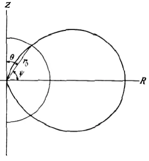
Fig. 3. Illustration of a Størmer orbit and the definition of the angle ϑ=90◦−ψ. The valuer0represents the Earth’s radius (Størmer, 1955).
co-latitudeϑ0it can be calculated by the simple relation (cf. Stern (1969) for a derivation)
L= 1
sin2(ϑ0)
. (13)
As illustrated in Fig. 2, Lis the distance in Earth radii, at which a magnetic field line penetrating the Earth’s surface at the co-latitudeϑ0 crosses the equatorial plane. Because of the fact that theLparameter is neither defined for a gen-eral planetary field, nor can be calculated even for the def-inition above, it must be computed indirectly. The tradi-tional method to do so employs the Størmer orbits in auro-ral latitudes. Carl Størmer’s work dealt with charged parti-cles penetrating into the Earth’s magnetic field at high lati-tudes, leading eventually to the formation of auroral lights. Therefore, he calculated the so-called forbidden and allowed particle trajectories of charged particles moving towards the Earth (Størmer, 1955). The origin of charged particles de-tected in the Earth’s magnetic field can be established by (nowadays numerically) retracing the particles’ trajectories back into the interplanetary space, rather than to compute the orbits towards the Earth. Forbidden orbits are those remain-ing close to Earth or returnremain-ing to it. The allowed ones are those along which the particles can actually escape. Such an Størmer orbit, where the distance, r, parameterised by the angleϑwithr0representing the Earth’s radius (cf. Fig. 3) is given by Størmer (1955) as
r=Cst· sin 2ϑ
1+p1+sin3ϑ
(14)
withr being given in Earth radii and the Størmer constant
Cst=
√
m/P, which contains the magnetic momentm=|m| of the Earth and the rigidity (momentum per charge)P of the particles.
Fig. 4. Comparison of the functions f1(ϑ )=sin2ϑ/2 and f2(ϑ )=sin2(ϑ )/(1+
p
1+sin3ϑ )withϑbeing the co-latitude.
Because Størmer was only interested in high latitudes, i.e. regions of small values ofϑ, he could neglect the sin3ϑterm in the denominator, leading to
r2= m 4P ·sin
4ϑ, (15)
giving a relation between the rigitityP that denotes a parti-cle’s momentum per unit charge, and theLparameter, if the latter is inserted according to Eq. (13) and evaluated on the Earth’s surface, i.e.r=r0, leading to
P=K· 1
L2, (16)
withK=m/(4r0)=14.81 GV.
A more realistic dependency was given by Shea and Smart (1986) by using a least-square fit of simulated and measured data. They found:
P= ˜K· 1
Lq (17)
with the slightly different values K˜=14.823 GV and
q=2.0311.
The traditional approach to compute theLparameter con-sists of performing numerical simulations or employing mea-surements in order to obtain the maximum rigidity, at which a particle can hit the Earth’s surface at a given latitude on an allowed orbit, the so-called cut-off rigidity, and relate the latter to the respectiveLparameter by means of Eq. (17). In order to calculate theLparameter along a trajectory or for a part of the Earth’s surface, the cut-off rigidity has, thus, to be known for every point along it.
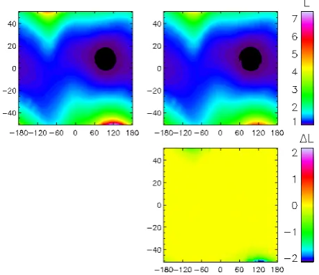
Fig. 5. Comparison between theLparameter calculated with the Tsyganenko89 (upper left panel) and IGRF (upper right panel) mod-els as a function of longitude and latitude. The bottom panel shows the difference between both models.
To check on the validity of this approximation, we plotted the simplified functionf1(ϑ )=sin2ϑ/2 and the full function f2(ϑ )=sin2(ϑ )/(1+
p
1+sin3ϑ )against the co-latitudeϑ, shown in Fig. 4.
The comparison shows the approximation to be valid only in auroral regions, corresponding to a latitude aboveψ≈60◦ (or co-latitudeϑ≈30◦), so that deviations between the de-rived and the calculatedLparameters are to be expected in particular in equatorial regions (cf. Sect. 3).
An example forLparameters derived with the relation by Shea and Smart (1986) by means of numerical simulations with the PLANETOCOSMICS code5, a GEANT based sim-ulation code, is shown in Fig. 5. The simsim-ulations were carried out for the IGRF model for 2008 as well as for a magnetic field perturbed by the Solar wind according to the Tsyga-nenko89 model (Tsyganenko, 1989) for the latitudinal range covered by the International Space Station, ISS. BothL pa-rameters show low values in equatorial regions with a mini-mum around a longitude of about 90◦and values up toL=6 in high latitudes. The whole structure shows a strong bend around a longitude of about−90◦. The comparison indicates significant differences between both magnetic field models (bottom panel) only in latitudes of 50◦ or higher. If theL
parameter is used to interprete data measured close to the Earth’s surface it is sufficient to use the IGRF model for the calculations of theLparameter in Sect. 3.
5http://cosray.unibe.ch/∼laurent/planetocosmics
simple method to calculate them numerically. As mentioned above, we use the IGRF model for 2008 in the following.
The IGRF model uses Eq. (4) with the coefficientsgnmand
hmn being derived from a network of observations every five years, at last 2005, from which the values for 2008 were ex-trapolated. These values as well as a numerical code can be accessed via the IGRF website http://www.ngdc.noaa.gov/ IAGA/vmod/igrf.html. In order to calculate theL parame-ters defined below, we used a simple algorithm to integrate magnetic field lines r=r(s)according to the relation r(s+δs)=r(s)+δs B(r(s))
|B(r(s))| (18) with the arc lengthsalong the field line and a fixed step size
δs. In order to evaluate the r.h.s., we modified the above men-tioned program in such a way that it provides the magnetic field components at the respective point in space. Simultane-ously, the following four criteria were evaluated during the integration:
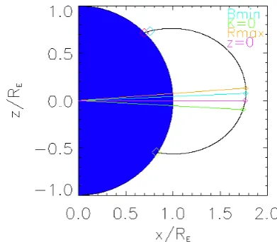
1. Minimal magnitude of the magnetic field (“Bmin”) We define the parameter L1 as that distance from the Earth’s centre at the point with the minimum magnetic field strength along the magnetic field line. Figure 6 il-lustrates this definition along an example field line. The colour along the field line gives the magnitude of the magnetic field, the black line points from the centre of the Earth to the point of minimum field strength. Its length, given in Earth radii, gives the value L1.
2. Passing the geomagnetic equator (“K= 0”)
The second parameter, L2, is defined as the distance at which a magnetic field line crosses the equatorial plane of the tilted dipole field (eccentric dipole) with dipole moment m and shift rq as described above. If r is the
vector defining L2, the scalar product
K=m·(r−rq) (19)
Fig. 6. Illustration of the first definition, L1, for theLparameter along a field line. The colour along the line shows the magnetic field strength. The colour table is the same as in Fig. 5. The red and green diamonds indicate the points, where the field line intersects the surface of the Earth. The field line is identified by the starting point of the integration, marked with a blue diamond.
Fig. 7. Same as Fig. 6 but for parameter L2, with the colour now showing the value ofK. Note that yellow indicates values close to zero.
3. Maximum distance (“Rmax”)
Parameter L3, the third possibility, is defined as the maximum distance from the centre of the Earth, which a point along a magnetic field line can attain and is shown in Fig. 8.
4. Passing the equatorial plane (“z= 0”)
Finally, L4 follows the tradional definition of McIlwain by the passage of a field line through the equatorial planez=0 (cf. Fig. 9).
All fourLparameters along the same field line are plotted together in Fig. 10. While the vector defining L4 (“z= 0”)
Fig. 8. Same as Fig. 6 but for parameter L3, with the colour now showing the distancer.
Fig. 9. Same as Fig. 6 but for parameter L4, with the colour now showing the distance of each point of the field line from the equato-rial plane.
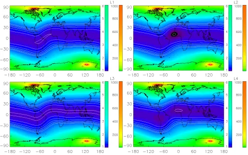
Fig. 11. MappedLparameters L1 (a), L2 (b), L3 (c) and L4 (d) for the geomagnetic IGRF model for 2008, plotted against the geographical longitude,ϕ, and latitude,ψ=90◦−ϑ. TheLparameter reach values of 1 up to 1000 as indicated in the color bars.
lies in the equatorial plane as expected, those for L1 (“Bmin”) and L3 (“Rmax”) are located close to each other above the equatorial plane, while that for L2 (“K= 0”) lies below it, re-flecting the local orientation of the tilted dipole field. Despite of the different locations of these four points, the lengths of the respective vectors and, thus, theLvalues are quite close to each other.
The results for L1 (a), L2 (b), L3 (c), and L4 (d) are plotted as a function of the geographical longitude and latitude in Fig. 11. In order to capture the large range ofLvalues from the equator towards the poles, theLparameters are shown here in a logarithmic scale.
For a better comparison and discussion of the four sug-gestedLparameters, we plotted the magnetic field compo-nents Br, Bϕ, and Bϑfor the 2008 IGRF model and the tilted
dipole in Figs. 12 and 13, respectively.
As already shown in Fig. 10 for a starting point at a lati-tude around 45◦, theLparameter may be defined by different vectors, but their values do not deviate much. This is, how-ever, not the case closer to the equator. Within latitudes of about±30◦, we observe larger differences in theL param-eters, while differences beyond this region become less vis-ible. The differences between the variousLparameters are caused by the geometry of the IGRF field:
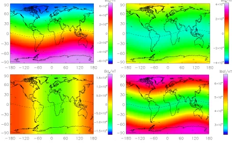
The parameters L1 and L3 hardly diverge from each other. It is interesting to note that their variation with longitude does not follow the geomagnetic equator (cf. Fig. 12a), but with the curveBr=0, i.e. the yellow line in Fig. 12a. Larger de-viations can be seen for L2, in particular, with a minimum above West Africa coinciding with the region, where the ra-dial component, Br, shows the largest differences between the IGRF field and the tilted dipole (cf. Fig. 12a for the IGRF model and Fig. 13a for the tilted dipole). For parameter L4 one can recognise the variation of the IGRF field around the equatorial planez=0 by structures above West Africa and South America (cf. Fig. 11d).
Fig. 12. IGRF field of the Earth in 2008 with the magnetic components Br (a), Bϑ (b), and Bϕ (c) as well as the magnitude|B|(d). The
dashed line shows the magnetic equator of the tilted dipole field.
well as by the very high rigidities corresponding to the low
Lparameters.
In order to understand the last point, we consider therand
ϑcomponents of the IGRF model, shown in Fig. 12a and b. We find a maximum inBϑ, which is located actually above
India, whereasBr takes very low values there. With respect
to the rigidities, this means that particles hitting the Earth’s surface in radial direction feel a magnetic field essentially perpendicular to their direction of motion, allowing only very energetic particles to reach the surface, leading to the ob-served high values for the cut-off rigidities. The latter, how-ever, merely reflect local field structures, but do not provide the required informations about the global one. Moreover, the rigidities do not fully take into account the other field components in this region as the direct computation does. Note, that also the feature of the magnetic field above India cannot be seen in the tilted dipole field (cf. Fig. 13).
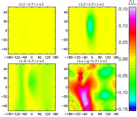
Furthermore, we show in Fig. 14 the relative differences between eachLparameter relating to the L3 parameter. The parameters L1 and L3 hardly diverge from each other (cf. Fig. 14a), whereas the deviation for L2 (b) and L4 (c) are mostly noticeable in the equatorial plane with a slightly dif-ference above India for L2. On the contrary, the deviation between L3 and the traditionalLparameter computed with the rigidities (d) is strong and varies for all latitudes, with the highest variation being 15%.
We may conclude that the traditional method does not in all regions reflect the magnetic field geometry, because it uses the indirect way via cut-off rigidities. Furthermore, the relation by Shea and Smart (1986), Eq. (17), is based on Størmer orbits performed for an aligned dipole. In particular, the Eq. (15) is valid only in higher latitudes (cf. Fig. 4). A further point is the fact that the values forK˜andqderived by Shea and Smart (1986) are based on data from the early 80s and thus cannot reflect the temporal evolution of the mag-netic field. Moreover, the new method allows to compute the
Lparameter along a certain orbit of a spacecraft for different altitudes. In addition, providing the cut-off rigidities with nu-merical methods or data is not only time-consuming, but also difficult for different altitudes and considerably more inaccu-rate, because a mesh with limited grid size has to be used.
Fig. 14. Relative difference between the L3 parameter and L1 (a), L2 (b), L4 (c) and the traditionalLparameter computed indirectly with the rigidities (d).
4 Summary and conclusions
An important quantity to identify the origin of particles in planetary magnetic fields is the L parameter, which so far has only been defined for an aligned dipole field and speci-fies the distance of a field line from the Earth’s centre in the equatorial plane measured in Earth’s radii. The latter was at first defined by McIlwain (1961) and thus is called the McIl-wain parameter, which at a given co-latitudeϑ0is given by the simple relationL=1/(sin2ϑ0). Up to now theL param-eter could only be assessed indirectly by employing cut-off rigidities,P, of energetic particles, taken e.g. from numerical simulations, which subsequently are related to the respective
Lparameter by means of the EquationP= ˜K/Lq. Such a relation was originially found by Størmer (1955) only for re-gions in high latitudes in an aligned dipole field. A more accurate relation was later derived by by Shea and Smart (1986). Therefore, not only a newer and direct method is neccessary to calculate theLparameter, but a general signif-icant definition for theLparameter is desirable as well. We successfully found a simple method, as well as four potential definitions of theLparameter for a realistic magnetic field described as:
1. L1 is defined as the distance from Earth’s centre at the point with the minimum magnetic field strength. 2. L2 describes the distance at which a magnetic field line
crosses the equatorial plane of the tilted dipole field with the dipole moment m and shift rq.
4. L4 follows the traditional definition of the McIlwain by the passage of a field line through the equatorial plane
z=0.
Since L2 and L4 rely on simplified magnetic field models (tilted and aligned dipole fields, respectively), but do not re-flect the geometry of the actual magnetic field, the parame-ters L1 and L3 appear to be the more appropriate definitions. From those we choose L3 as the most applicable definition for a realistic magnetic field, because compared to L1 it con-tains information about the excursion of the respective field line.
Comparing the traditional method with our new method we recognise large deviations, mostly in equatorial regions, that are caused at first by the use of the cut-off rigidities and second by simpifying, but at least partially inaccurate approximations leading to the relationP= ˜K/Lq. By em-ploying the latter relation to obtain theLparameter by the traditional, quite cumbersome method, only parts of the ge-omagnetic structure can be reflected compared to the new, direct computation that provides required information about the global geomagnetic structure.
The defintion of theLparameter as the maximum distance along a magnetic field line and the method to calculate it al-lows for the first time to describe charged particles linked to magnetic field lines in an actual and realistic planetary mag-netic field, in particular also for other planets in the Solar System.
Acknowledgements. This paper was partially financially supported by the Deutsche Forschungsgesellschaft, DFG, via the project CAWSES (He 3279/8-2 and 8-3).
Edited by: H.-J. Fahr
Reviewed by: two anonymous referees
References
Connerney, J.: Magnetic fields of the outer planets, J. Geophys. Res., 18, 659–679, 1993.
Gauss, C. F.: Allgemeine Theorie des Erdmagnetismus: Resul-tate aus den Beobachtungen des magnetischen Vereins im Jahre 1836, G¨ottinger Magnetischer Verein, Leipzig, 1–52, 1836. McIlwain, C. E.: Coordinates for Mapping the Distrubution of
Mag-netically Trapped Particles, J. Geophys. Res., 66, 3681–3691, 1961.
Roederer, J., Welch, J., and Herod, J.: Longitude dependence of geomagnetically trapped electrons, J. Geophys. Res., 72, 4431– 4447, 1967.
Shea, M. and Smart, D.: Estimating cosmic ray vertical cutoff rigidities as a function of the McIlwain parameter for different epochs of the geomagnetic field, Phys. Earth Planet. Interiors, 48, 200–205, 1986.
Stern, D. P.: Euler Potentials, Am. J. Phys., 4, 494–501, 1969. Størmer, C.: Polar Aurora, Clarendon Press Oxford, 294 pp., 1955. Tsyganenko, N.: A magnetospheric magnetic field model with a