The Effect of Sample Size On (Cusum and ARIMA) Control Charts

(1)

Infogain Publication (Infogainpublication.com) ISSN: 2454-1311

www.ijaems.com Page

|

397

The Effect of Sample Size On (Cusum and

ARIMA) Control Charts

Dr. Kawa M. Jamal Rashid

Ass. Prof , Department of Statistics,College of Administrations and Economics, Sulamani University, Sulamani, Kurdistan, Iraq

Abstract— The purpose of this paper is to study Statistical

Process Control (SPC) with a cumulative sum CUSUM chart which shows the total of deviations, of successive samples from the target value and the Average Run Length (ARL) is given quality level is the average number of samples (subgroups) taken before an active signal is given. Sample size has a good effect on the quality chart. The average run length of the cumulative sum control chart is the average number of observations that are entered before the system is declared out of control. Control limits for the new chart are computed from the generalized ARL approximation, The Autocorrelation of the observation increasing by the sample size of the cumulative value distributed by Manhattan diagram. The new chart is compared to other distribution-free procedures using stationary test processes with both normal and abnormal marginal.

Keywords— Cumulative sum CUSUM Chart, ARIMA Control chart, Average Run Length, Distribution-Free Statistical Methods, Manhattan diagram.

I. INTRODUCTION

Quality control via the use of statistical methods is a very large area of study in its own right and, is central to success in modern industry with its emphasis on reducing costs while at the same time improving quality, Statistical quality control came from Dr. Walter Shewhart in 1924 during his employment at Bell Telephone Laboratories. He recognized that in a manufacturing process, there will always be variation in the resulting products. He also recognized that this variation can be understood, monitored, and controlled by statistical procedures. Shewhart developed a simple graphical technique - the control chart - for determining if the product variable is within acceptable limits. In this case the production process is said to be in "control" and control charts can indicate when to leave things alone or when to adjust or change a production process. In the latter cases the production process is said to be out of control.’ Control charts can be used (importantly) at different points within the production process. [4]

The aim of statistical process control is to ensure that a given manufacturing process is as stable. In short, the aim is the reduction of variability to ensure that each product is of a high a quality as possible. Statistical process control is usually thought of as a toolbox whose contents may be applied to solve production-related quality control problems. [4] [3]

II. CUMULATIVE SUM CUSUM CHART

The basic Principles The Cusum control chart for monitoring the process mean.

The development of cumulative sum (CUSUM) control charts originally introduced by Page [1954]. The CUSUM control chart is a procedure based on the CUSUM of the deviations of the sample statistics from the target value [7]. Over the years, CUSUM control charts have proven to be superior to the classical Shewhart control charts in the sense that the CUSUM control charts tend to have smaller Average Run Lengths (ARL’s) particularly when small changes in the population parameters of the process have occurred [1].

∑

=

−

=

i

j j i

X

CUSUM

1

0

)

(

µ

…. (1)

Where the initial value of the cumulative statistics is taken to be zero [7].

To compute the upper and lower cumulative statistics, we now need the value of the reference value of k or (slack value). In our situation, ∆u is specified to be (0.01)

implying k is (=∆/2). Then k is computed by using

σ

ˆ

The tabular Cusum works by accumulating derivations from

µ0 that are above target with one statistic

Cusum

+and the below target with other statistics. The statistics

+

Cusum

and

Cusum

− are called one –sided upper and

lower Cusum. They are computed as follows:

{

}

{

+

}

− +

+ − +

+

−

=

+

−

=

1 0

)

(

,

0 max

CUSUM

)

(

,

0 max

CUSUM

i i

i

C

X

k

C

k

X

µ

(2)

|

398

Where the starting the value are

0

=

0

=

0

− +

C

Adjustment to some manipulatable variable is required in

order to bring the process back to the target value

µ

₀ this

can be computed as:[2][9]





















>

−

>

+

=

− +

−

+ +

+

H

C

if

N

C

k

H

C

if

N

C

k

i i

0 0

ˆ

µ

…3

III. PRODUCT SCREENING AND PER-SELECTION Cusum chart can be used in categorizing process output. This may be for the purposes of selection for different process or different assembly operation. The Cusum chart has been divided into different sections of average process mean by virtue of a change the slope of Cusum plot. The average process calculated as:

)

4 ...(

/

)

(

₁

1

n

S

T

n

X

i n n

i i

− =

−

+

=

∑

Where S is a Cusum value this information may be represented on a Manhattan diagram- [4]

IV. ARIMA CONTROL CHART

Classical Shewhart SPC concept assumes that the measured data are not autocorrelated.

Even very low degree of autocorrelation data causes failure of classical Shewhart control charts.

Failure has a form of a large number of points outside the regulatory limits in control diagram.

This phenomenon is not unique in the case of continuous processes, where the autocorrelation data given by the inertia processes in time. Autocorrelation of data becomes increasingly frequent phenomenon in terms of discrete processes, a high degree of automation of production and also in the test and control operations.

One of the ways to tackle autocorrelated data is the concept of stochastic modeling of time series using autoregressive integrated moving average models, the ARIMA model. Linear stochastic autoregressive models (models AR), moving average (model MA), mixed models (the ARMA models), and ARIMA models, based on Box-Jenkins methodology is seen as a time series realization of stochastic process [8][9] These models have a characteristic shape of the autocorrelation fiction (Autocorrelation Fuction–ACF) and partial autocorrelation function (Partial Autocorrelation Function – PACF). The original integrated

process is called an autoregressive integrated moving average process of order p, d, q, ARIMA (p, d, q) where p number of autoregressive terms, d is number of nonseasonal differences, and q is a number of moving – average terms.

Location of the mean value CL and upper and lower control limits (UCL, LCL) for the ARIMA (p,d,q) chart for individual values can be determined from the formula as:

i

x

R

X

LCL

and

UCL

x

CL

128 .

1

3

0 m

=

x

: Is the average of residual value.

R

: Is the average of moving rang.

Values CL, UCL and LCL can be calculated as follows.

0

267 .

3 =

=

LCL

R

UCL

R

CL

i

x

To increase the sensitivity of control charts ARIMA is recommended to use two-sided Cusum control chart with the decision interval ± H. .[8][9][11]

V. AVERAGE RUN LENGTH - ARL Any sequence of samples that leads to an out-of-control signal is called a “run.” The number of samples that is taken during a run is called the “run length.” The use of Average Run Length (ARL) has considerable fire in recent years .This is because the run length distribution is quite skewed so that the average run length will not be a typical run length, and the another reason that is the standard deviation of the ARL is quite large, and as Geometric distribution, the variance of geometric distribution.[10]

The term Average Run Length (ARL) is defined as the average or expected number of sizes in the process level is signaled by points that must be plotted before an out-of-control.

If (p) is the probability of a single plotted point breaching the predetermined control limits (signaling a lack of statistical control), then the ARL is given by the mean of the geometric distribution namely.

For attribute and variables Shewhart charts with only three sigma action or control limits, the probability p is assumed to be constant

For a Shwhart - type chart the ARL for a in control process

typically labeled

ARL

₀ is given by;

α

1

0

=

(3)

|

399

-0.800 -0.700 -0.600 -0.500 -0.400 -0.300 -0.200 -0.100 0.000 0.100 0.200 0.300 0.400

1 3 5 7 9 11 13 15 17 19 21 23 25 27 29 31 33 35 37 39 41 43 45 47 49 51 53 n=3

n=4

n=5

n=6

And the probability of getting an out-of-control signal if the process has shifted is β, then the processes is out of control

as

ARL

₁ is:

β

α

−

=

−

=

−

=

∑

∞ = −

1

1 )

(

1

1 )]

(

1 [

)

(

1 1 1

P

iP

ARL

i i

Where α is the probability of a Type I error and β the probability of a Type II error. [6][7]

VI. TABULAR CUSUM PROCEDURE FOR MONITORING THE PROCESS MEAN The Tabular Cusum is designed by choosing values for the reference value K, and the decision interval H. These parameters be selected to provide a good average run length performance. The parameter H defines as H=hσ and K= hσ where σ is the standard deviation of the samples used in forming the Cusum. Using h=4 or h=5 and k=0. 5 a custom that has a good ARL property against a shift of about 1σ in the process mean.[2] -

ARL

Approximation for upper-side CUMUM

ARL

+

and lower –side CUMSE

ARL

− are given by:

[

]

)

(

2

1 )

166 .

1 )

(

2 )

166 .

1 )(

(

2 exp

k

h

k

h

k

ARL

_u u u

−

+

−

+

−

=

+

δ

…4 And

[

]

)

(

2

1 )

166 .

1 )(

(

2 )

166 .

1 )(

(

2 exp

k

h

k

h

k

ARL

_u u u

−

+

−

+

−

=

−

δ

.… (5)

And the ARL for two sided Cusum can be obtained by using the following as:

− + − +

=

+

ARL

1

, …(6)

From Eq. (5) If the value of (k) is equal (0.5) then the value of (h) is equal (4.767), and ARL is(370) [6][7]

VII. NUMERICAL STUDIES

Numerical illustration: In this section an application is considered to highlight the features of the above proposed Cusum control charts. In this paper through a rea illustrative data from ALA-Company for bottle water.The application was made in controlling the proportion of (Power of Hydrogen) PH component in the water. Thirty two samples with a sample size of 5 (the total measurement number is 160) were taken from the production process in the ALA Company as shows in table (4). These measurement data are converted into trapezoidal Cusum numbers and given in Table (1). Designing and determine calcium control chart

for a process average of variable quality. Table (2) shows that the value of the Cusum stat chart for the sample size n= (3, 4, 5, 6) as shows in Fig (1, 2, 3 and 4)

Table (1) Cusum Value of PH For different sample size n

Sample Size n=3 Sample size n=4 Sample size n=5 Sample size n=6 -0.024 -0.040 -0.024 -0.029

-0.059 0.040 0.063 0.055

0.077 0.082 0.057 -0.008

0.109 0.044 -0.023 -0.019

0.095 -0.028 -0.030 0.168

-0.016 -0.029 0.202 0.081

. . . .

-0.347 -0.329 -0.259 -0.214 -0.305 -0.354 -0.282 -0.215 -0.239 -0.289 -0.278 -0.233 -0.140 -0.219 -0.274 -0.236 -0.118 -0.179 -0.175 -0.173 -0.185 -0.094 -0.129 -0.120 -0.146 -0.120 -0.071 -0.059 0.003 -0.110 -0.106 -0.073

-0.005 0.000 0.000 0.037

Fig.1:Cusum distribution of sample size (n, 3,4,5,6)

Fig.2:Cusum stat distribution sample size n= 3

Samplie size n-3

-0.3 -0.2 -0.1 0 0.1 0.2 0.3 0.4 0.5

(4)

|

400

Table (2) Basic statistic table

Sample

size n=3

Sample size n=4

Sample size n=5

Sample size n=6

Minimum -0.194 -0.14 -0.122 -0.111

Maximum 0.396 0.262 0.232 0.187

Range 0.59 0.403 0.354 0.298

Standard

Deviation 0.09 0.073 0.075 0.068

Variance 0.008 0.005 0.006 0.005

Fig.6:Manhattan diagram for the average process mean

From Fig. (1,2,3,4 and5) and the basic statistic table shows that the Cusum value has a different range of Cusum value, each case depends upon the sample size n, the range of Cusum stat is equal (0.298) if sample size is (n=3) and the range is equal (0.59) if sample size is (n=6), with variance (0.005, 0.008) it means that decreasing the deviation between our observations or the rang value of Cusum by increasing the sample size. In designing a control chart, we must specify both the sample size and the frequency of sampling. In general, larger samples will make it easier to detect small shifts in the process, The Cusum rang value depend upon the sample size of these deviations, Cusum is particularly helpful in determining when the assignable cause has occurred, as we noted in the previous example, just count backward from the out-of-control signal to the time period when the Cusum lifted above zero to find the first period following the process shift. We conclude that sample size has a good effect on a control chart. In some situations where an adjustment to some main table variable is required in order to bring the process back to the target value m0, it may be helpful to have an estimate of the new process mean following the shift. The counters N+ and N- are used in adjustment.

This can be computed from by equation (3) we would estimate the new process average of

4 .

6

54 .

7

9

=

− +

C

and

C

We would conclude that mean shifted from 7 to 7.54, then we would need to make an adjustment in PH rate by 0.54 units, to estimating the mean of any we would conclude that mean. By using the Average process for Cusum for Sample Size 5

-0.15 -0.1 -0.05 0 0.05 0.1 0.15 0.2 0.25 0.3

1 4 7 10 13 16 19 22 25 28 31 34 37 40 43 46 49 52

Sample size 6

-0.15 -0.1 -0.05 0 0.05 0.1 0.15 0.2 0.25

1 4 7 10 13 16 19 22 25 28 31 34 37 40 43 46 49 52

Sample size 4

-0.2 -0.15 -0.1 -0.05 0 0.05 0.1 0.15 0.2 0.25 0.3

(5)

|

401

different sample size, from the fig. (6). It shows that the variation in average process means in sample size n=6 is approach to equal time –scale it shows that chart with sample size n=6 have more stable distribution.

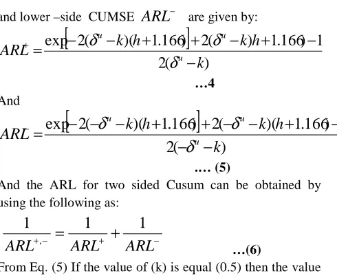
Fig.7:ARIMA control chart.

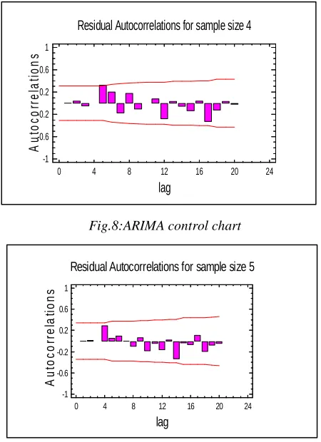
From Fig. (7, 8 , 9 and 10) it shows that the sample size has an effective on the ARIMA control chart the Fig.(10) have a more effective than Fig.(7) where the sample size (n=3)

Fig.8:ARIMA control chart

Table (3) UCL, LCL, Mean and variance If N= 3,4,5,6

Table (4) ARIMA Model Summary

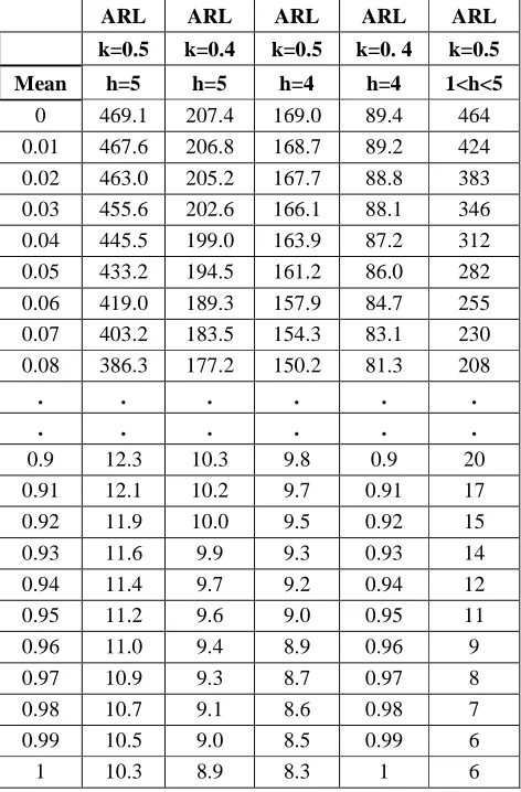
In this paper determining the Average Run Length ARL of PH parameter of water defining the ARL by different type of parameter (K, and H) as shows in table (3) and ARL distribution as Fig. (11). We must also determine the frequency of sampling. The most desirable situation from the point of view of detecting shifts would be to take large samples very frequently; however, this is usually not economically feasible. Define H= hσ and K= kσ, where σ is the standard deviation of the sample. Calculating the ARL for different value of a parameter (k (0.5, 0.4,) and h (5, 4)) with shift mean as shows in table and Fig. (12), although determining the ARL with k=0.5 and changing the h from 1 to 5, if the value of parameter h= 4.77 this will provide ARL0 = 370 samples as shows in table(5) and Fig. (11and 12).

ARIMA

Chart

N=3 N=4 N=5 N=6

UCL 0.158 0.1117 0.1025 0.0854 LCL -0.158 -0.1117 -0.1025 -0.085 Mean 7.0075 7.0076 7.0088 7.007 St dev 0.1567 0.14902 0.1702 0.1733

ARIMA

Parameter Estimate

Stand. Error t

P-value

Sample 3 0.0633 0.13831 0.458 0.648

Sample 4 -0.0096 0.16651 -0.057 0.954

Sample 5 -0.1691 0.18581 -0.910 0.37

Sample 6 -0.1691 0.18581 -0.910 0.37

Residual Autocorrelations for n=3

lag

A

u

to

c

o

rr

e

la

ti

o

n

s

0 4 8 12 16 20 24

-1 -0.6 -0.2 0.2 0.6 1

Residual Autocorrelations for sample size 4

lag

A

u

to

c

o

rr

e

la

ti

o

n

s

0 4 8 12 16 20 24

-1 -0.6 -0.2 0.2 0.6 1

lag

A

u

to

c

o

rr

e

la

ti

o

n

s

0 4 8 12 16 20 24

-1 -0.6 -0.2 0.2 0.6 1

lag

A

u

to

c

o

rr

e

la

ti

o

n

s

0 4 8 12 16 20 24

(6)

|

402

40 36 32 28 24 20 16 12 8 4 500

400

300

200

100

0

k=0.5 and h =5 to 1

Fig.11:ARL Distribution with value K and H

Table (5) ARL value with different (K, and h)

ARL ARL ARL ARL ARL

k=0.5 k=0.4 k=0.5 k=0. 4 k=0.5

Mean h=5 h=5 h=4 h=4 1<h<5 0 469.1 207.4 169.0 89.4 464 0.01 467.6 206.8 168.7 89.2 424

0.02 463.0 205.2 167.7 88.8 383 0.03 455.6 202.6 166.1 88.1 346 0.04 445.5 199.0 163.9 87.2 312 0.05 433.2 194.5 161.2 86.0 282

0.06 419.0 189.3 157.9 84.7 255 0.07 403.2 183.5 154.3 83.1 230 0.08 386.3 177.2 150.2 81.3 208

. . . . . .

0.9 12.3 10.3 9.8 0.9 20

0.91 12.1 10.2 9.7 0.91 17 0.92 11.9 10.0 9.5 0.92 15

0.93 11.6 9.9 9.3 0.93 14

0.94 11.4 9.7 9.2 0.94 12

0.95 11.2 9.6 9.0 0.95 11

0.96 11.0 9.4 8.9 0.96 9

0.97 10.9 9.3 8.7 0.97 8

0.98 10.7 9.1 8.6 0.98 7

0.99 10.5 9.0 8.5 0.99 6

1 10.3 8.9 8.3 1 6

Fig.12:ARL distribution k=0.5 and h=5

VIII. SUMMARY AND CONCLUSIONS In this paper investigates the limitations of the traditional concept of the Cusum and average run length, it is seen that the Cusum chart is a good technique and have a small sift between the observation and the sample size n have a good estimate on the Cusum and ARL. The ARL distribution affected by the parameter value of k and h, so in the best ARL graph is if value of k=5, and h=5 Decreasing the deviation and range between our observations by increasing the sample size (subgroup).In designing a control chart, we must specify the sample size in determining Cusum value. In general, larger samples will make it easier to detect small shifts in the process. The Cusum chart is particularly helpful in determining when the assignable cause has occurred, effective

Table (6) proportion of PH in Water for 32 days

PH N. of

Day X1 X2 X3 X4 X5

1 6.97 6.88 6.76 6.8 7.02 2 7.02 6.86 7 6.82 6.92 3 6.96 6.8 7.05 6.82 7.03 4 6.92 6.97 6.9 7.03 6.96 5 7.05 6.96 6.67 6.92 6.97 6 6.95 6.97 6.91 6.99 7 7 7.34 7.17 7.22 7.11 7.1 8 7.01 6.88 7.1 7.05 7.22 9 7.08 7.03 7.06 7.17 7.07 10 7.09 7 7.04 7.08 7.06

. . . . . .

(7)

|

403

26 6.9 6.84 6.84 6.84 6.96 27 7.09 6.93 7.02 7 7.08 28 7.14 6.97 7.06 7.06 7.1 29 7.12 7.02 6.86 7.09 7.39 30 7.95 6.95 7.02 7.02 7.06 31 7 7.09 7.06 7.12 7.02 32 7.01 6.97 6.96 6.98 7

REFERENCES

[1] Arthur B. Yeh , Dennis K. J. Lin (2004) , Quality Technology & Quantitative Management Vol.1, No.1 pp. 65-86, 2004 Unified CUSUM Charts for Monitoring Process Mean and Variability”

[2] Douglas C. Montgomery 2009, Introduction to Statistical Quality Control 6th edition.

[3] Getulio Rodrigues De Olivera Filho, MD (2000) Economics, Education, And Health System Research 2002 . Construction of Learning Curves for basic skills in Anesthetic Procedures An Application for the Cumulative Sum Method

[4] John Oakland 2008 Statistical Process Control, Sixth Edition.

[5] HELM (VERSION 1: April 8, 2004): Workbook Level 1 46.2: Quality Control

[6] KARAOGLAN A.D. and BAYHAN G. M. March 2012; ARL performance of residual control charts for trend AR (1) process: A case study on peroxide values of stored vegetable oil Department of Industrial Engineering, Balikesir University, Cagis Campus, 10145, Balikesir -Turkey.

[7] Layth C. Alwan 2000 “Statistical Process Analysis [8] M. Kovářík, Klímek Petr (2012) The Usage of Time

Series Control Charts for Financial Process Analysis, Journal of Competitiveness Vol. 4, Issue 3, pp. 29-45, September 2012 ISSN 1804-171X (Print), ISSN 1804- 1728 (On-line), DOI: 10.7441/ joc. 2012.03.03

[9] M. Kovářík, 2013: Volatility Change Point Detection Using Stochastic Differential Equations and Time Series Control Charts, Issue 2, Volume 7, 2013,

INTERNATIONAL JOURNAL OF

MATHEMATICAL MODELS AND METHODS IN APPLIED SCIENCES

[10]Ryan T.P (2000) : ( Statistical Methods For Quality Improvement), 2end Edition-

[11]Sermin E., Nevin U. And Mehemt S. Oct. 2008 Control Charts for qutocorrelated d claimant data [12]Journal Of scientific & Industrial Research Vol.68