Distance-Vector Algorithms for Distributed Shortest
Paths on Dynamic Power-Law Networks
Mattia D’Emidio1,* and Daniele Frigioni2,*
1 Gran Sasso Science Institute (GSSI), Viale Francesco Crispi, I–67100 L’Aquila, Italy
2 Department of Information Engineering, Computer Science and Mathematics, University of L’Aquila, Via Vetoio,
I–67100 L’Aquila, Italy
* Correspondence: [email protected] (M.D.); [email protected] (D.F.)
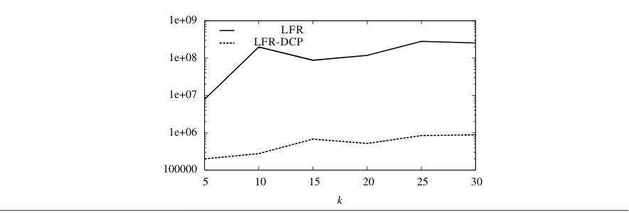
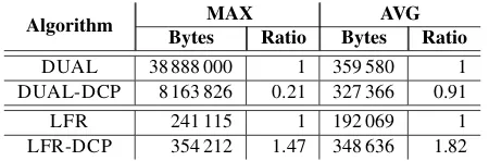
Abstract: Efficiently solving the problem of computing, in a distributed fashion, the shortest paths of a graph whose topology dynamically changes over time is a core functionality of many today’s digital infrastructures, probably the most prominent example being communication networks. Many solutions have been proposed over the years for this problem that can be broadly classified into two categories, namelyDistance-Vectorand Link-Statealgorithms. Distance-Vector algorithms are widely adopted solutions when scalability and reliability are key issues or when nodes have either limited hardware resources, as they result in being very competitive approaches in terms of both the memory and the computational point of view. In this paper, we first survey some of the most established solutions of the Distance-Vector category. Then, we discuss some recent algorithmic developments in this area. Finally, we propose a new experimental study, conducted on a prominent category of network instances, namelygeneralized linear preference(GLP) power-law networks, to rank the performance of such solutions.
Keywords: dynamic algorithms; distributed shortest paths; communication networks; routing protocols; power-law networks
1. Introduction
Efficiently solving the problem of computing, in a distributed fashion, the shortest paths of a graph whose topology dynamically changes over time is a core functionality of essentially all modern digital infrastructures, probably the most prominent example being communication networks. For this reason, the problem has been widely investigated in past decades and many solutions have been proposed over the years, which can be broadly classified into two categories, namelyDistance-VectorandLink-Statealgorithms, depending on the way they achieve the computation of shortest paths [1–5].
On the one hand, Distance-Vector algorithms, such as, e.g., theDistributed Bellman-Ford(DBF) method [3], are characterized by alocalnature, in the sense that a generic node executing this kind of algorithms usually interacts only with its neighbors and stores minimal little information about the global status of the network. In more details, typically, each node performing a Distance-Vector algorithm maintains only a single data structure (most of the times referred to asrouting table) containing, for each other node of the network, thedistance, i.e. the weight of a shortest path, and thenext hop, i.e. the next node on the same shortest path. Note that, this is, in general, the essential information regarding shortest paths to be stored in most of the applications of interest, like e.g., in data routing where the next hop is used to forward data toward destination nodes of interest.
The computation (and the maintainance under dynamic settings) of the routing table is, in the case of Distance-Vector algorithms, performed by solving very simple equations (see [6] and references therein), thus making them very competitive solutions from thecomputational complexitypoint of view. However, Distance-Vector based protocols, in dynamic scenarios, can suffer from some well-known and undesired phenomena, namelyloopingandcount-to-infinity, that can heavily affect their performance in terms of usage of communication resources (a.k.a.messageorcommunication complexity), tough quite efficient countermeasures for such issues are known.
On the other hand, Link-State algorithms, as for example the widely adoptedOpen Shortest Path First (OSPF) protocol [2], are characterized by aglobalnature, as they require each node to store the entire network
topology. Shortest paths, in this case, are usually computed by running a centralized shortest path algorithm, as for example the classic Dijkstra’s algorithm [7]. This results in a usage of memory (a.k.a.space complexity) which is asymptotically quadratic in the number of nodes of the network, in contrast to the linear requirements of Distance-Vector algorithms. On the positive side, Link-State approaches do not incur in looping and count-to-infinity phenomena, thus being, in static environments, more competitive w.r.t. Distance-Vector algorithms in terms of communication complexity. However, this is counterbalanced in dynamic scenarios, where they perform quite poorly in this sense, since each node needs to receive and store up-to-date information on the entire network topology after any change. This is achieved by broadcasting each modification affecting the network topology to all nodes [2,8,9], and by using a centralized algorithm for dynamic shortest paths, as for example those proposed in [10,11].
In the last few years, there has been a renewed interest in devising new efficient and light-weight distributed shortest-path algorithms for large-scale networks (see, e.g., [6,12–19] and references therein), where Distance-Vector algorithms has been considered as an attractive alternative to Link-State solutions either when scalability and reliability are key issues or when the memory/computational resources of the nodes of the network are limited.
The great majority of Distance-Vector solutions known in the literature (see, e.g., [1,20–24]) are based on the above mentioned DBF, introduced for the first time in Arpanet in the late 60’s [25], and still used in some real-world networks, as a part of the RIP protocol [8]. DBF is known to converge to the correct distances (and thus to be able to compute next-hops correctly) if the link weights stabilize and all cycles have positive lengths [26]. However, the convergence time can be very high (and possibly infinite) due to theloopingand count-to-infinityphenomena. Furthermore, if the nodes of the network are not synchronized, even when no change occurs in the network, the overall number of messages sent by DBF is, in the worst case, exponential with respect to the size of the network [27].
Among Distance-Vector algorithms, probably the most prominent one is DUAL (Diffuse Update ALgorithm), proposed for the first time in [5] and part of CISCO’s widely usedEnhanced Interior Gateway Routing Protocol(EIGRP) [28]. DUAL is more complex with respect to the baseline DBF since it uses, besides the routing table, several auxiliary data structures to guarantee freedom from looping and count-to-infinity phenomena. Another loop-free Distance-Vector algorithm that is worth to be mentioned isLoop Free Routing (LFR), which has been more recently proposed in [29]. Asymptotically, LFR has the same theoretical message complexity of DUAL but it uses an amount of data structures per node which is always smaller than that of DUAL. From the experimental point of view, LFR has been shown in [29] to be very effective in terms of both the number of messages sent and the memory requirements per node in some real-world networks of particular interest.
Internet Data Analysis(CAIDA) [31], an association that provides data and tools for the analysis of the Internet infrastructure; ii) synthetic topologies generated by theBarabási-Albertalgorithm [32].
In this paper, we first survey the main features of some of the most established solutions of the Distance-Vector category, namely DBF, DUAL, and LFR. Then, we summarize the main characteristics of DCP. Finally, we assess, via an extensive experimental evaluation, the performance of DUAL, LFR and their combinations with DCP, and provide evidences of its effectiveness, on a practically relevant class of power-law networks, namely power-law artificial instances obtained by the Generalized Linear Preference (GLP) model [33]. The GLP framework has been shown, by many studies focusing on distributed algorithms (see, e.g., [34,35]) to model very well the Internet, and parts of it. In particular, in [36], it has been shown that GLP predicts the structure of real-world communication networks (e.g. the Internet) better than the Barabási–Albert linear preferential model. This behaviour is better captured by the GLP model which adds more flexibility than Barabási–Albert in specifying how nodes connect to other nodes. The results of our experimental evaluation can be summarized as follows: given a generic Distance-Vector algorithmA, we provide strong evidences that combining it with DCP, in GLP network topologies, allows: i) a huge reduction (a couple of orders of magnitude in most of the cases) in the utilization of communication resources (measured in terms of messages sent) with respect toAwithout DCP; ii) a significant improvement in terms of memory requirements with respect toA without DCP. As a side result, the experiments also show that LFR outperforms DUAL in terms of number of messages sent and is very effective from the memory requirements point of view in GLP networks.
The paper is organized as follows. In Section2we give all the necessary background and notation. In Sections3,4and5we review DBF, DUAL, and LFR, respectively. In Section6we describe DCP and its combinations with both DUAL and LFR, and overview the experimental study of [30]. In Section7we show the results of our new experimental study on the GLP power-law networks. Finally, Section8concludes the paper.
2. Background
In this section, we provide all the necessary background and notation that will be used through the paper. We consider the classic distributed scenario where we have a network made of processors that are connected through (bidirectional) communication channels and exchange data using a message passing model, in which:
• each processor can send messages only along its own communication channels, i.e. to processors it is connected with;
• messages are delivered to their destination within a finite delay;
• there is no shared memory among the processors;
• the system isasynchronous, that is a sender of a message does not wait for the receiver to be ready to receive the message. The message is delivered within a finite but unbounded time.
Moreover, we assume the system to be asynchronous, as well as that described in [37], which is briefly summarized below. Thestateof a processorvis the content of the data structure stored byv. Thenetwork stateis the set of states of all the processors in the network plus the network topology and the channel weights. Aneventis the reception of a message by a processor or a change to the network state. When a processorpsends a messagem to a processorq,mis stored in a buffer located atq. Whenqreadsmfrom its buffer and processes it, the event “reception ofm” occurs. Messages are trasmitted through the channels inFirst-In-First-Out (FIFO)order, that is, messages arriving at processorqare always received in the same order as they are sent byp. Anexecutionis a (possibly infinite) sequence of network states and events. A non-negative integer number is associated to each event, thetimeat which that event occurs. Time is aglobalparameter and is not accessible to the processors of the network. Moreover, time must be non-decreasing and must increase without any bound, if the execution is infinite. Finally, events are ordered according to the time at which they occur. Several events can happen at the same time as long as they do not occur on the same processor. This implies that the times related to a single processor are strictly increasing.
2.1. Graph Notation
a weight functionw:E→R+that assigns to each edge a real value representing the optimization parameter
associated to the corresponding channel, such as, e.g. the time needed to traverse the corresponding link if a packet is sent on it. Given a graphG= (V,E,w), we will denote by:(v,u)an edge ofEthat connects nodes v,u∈V, and byw(v,u)its weight, respectively; N(v) ={u∈V :(v,u)∈E}the set of neighbors of a node v∈V;deg(v) =|N(v)|the degree ofv, for eachv∈V;maxdeg=maxv∈Vdeg(v)the maximum degree among
the nodes inG. Furthermore, we will use{u,. . .,v}to represent a generic path inGbetween nodesuandvand, given a pathP, we will usew(P)to denote itsweight, i.e. the sum of the weights associated to its edges. A path P={u, ...,v}is called ashortest pathbetweenuandvif and only ifPis a path having minimum weight among all possible paths betweenuandvinG. Given two nodesu,v∈V, we will denote byd(u,v)the topological distancebetweenuandv, i.e. the weight of ashortest pathbetweenuandv. Finally, we will callvia(u,v)the viafromutov, i.e. the set of neighbors ofu(there might be more than one) that belong to a shortest path fromu tov. More formally,via(u,v)≡ {z∈N(u)|d(u,v) =w(u,z) +d(z,v)}.
2.2. Performance Model
As shown in [38], the performance of a distributed algorithm in the asynchronous model depend on the time needed by processors to execute the local procedures of the algorithm and on the delays incurred in the communication among nodes. These parameters heavily influence the scheduling of the distributed computation and hence the number of messages sent. For these reasons, to properly analyze the behaviour of the solutions described in this paper with respect to convergence time, in what follows we consider the so-called FIFOnetwork scenarioas it is universally considered the most suited for analyzing the performance of distributed algorithms in the considered setting.
The FIFOnetwork scenario can be briefly summarized as follows: the weight of an edge models the time needed to traverse the corresponding link (the delay occurring on that edge if a packet is sent on it) and all the processors require the same time to process every procedure (the delay occurring on a processor if a procedure is performed on it), which is assumed to be instantaneous. In this way, the distance between two nodes models the minimum time that such nodes need to communicate. Then, the time complexity is measured as the number of steps performed by the processors, that is the number of times that a processor performs a procedure.
In this paper, we concentrate on the realistic case ofdynamic networks, i.e. networks that vary over time due to change operations occurring on the processors or on the communication channels, respectively. We denote a sequence of update operations on the edges of graphGrepresenting the network byC = (c1,c2, ...,ck). Assuming
G0≡G, we denote byGi, 0≤i≤k, the graph obtained by applyingcitoGi−1. Without loss of generality, we restrict our focus on the case where operationcieither increases or decreases the weight of an existing edge in
Gi, as insertions and deletions of nodes and edges can be easily modelled as weight changes (see, e.g., [6] for
more details). Moreover, we consider the case of networks in which a change in the weight of an edge (either increase or decrease) can occur while one or more other edge weight changes are under processing. A processor vof the network might be affected by a subset of these changes. As a consequence,vcould be involved in the concurrentexecutions related to such changes. We will usewt(),dt(), andviat()to denote a given edge weight, distance, or via in graphGt, respectively.
2.3. Complexity Measures
In the remainder of the paper, the performance of some of the considered algorithms will be measured in terms of two parameters, namelyδ and∆, which have been considered in several works on the matter (see, e.g. [5,20,21,29] and reference therein) since they capture pretty well the amount of distributed computation that has to be carried out to update the shortest paths in dynamic networks, as a consequence of one or more update operations.
In more details, given a sequenceC = (c1,c2, ...,ck)of update operations, we define parameterσci,sto represent, for each operationciand for each nodes, the set of nodes that change either the distance or the via
towardsas a consequence ofci. More formally, such parameter is defined as
σci,s={v∈V|d
If a nodev∈ ∪k
i=1{∪s∈Vσci,s}, thenvis said to beaffected. We denote by∆the overall number of affected nodes,∆=∑ki=1∑s∈V|σci,s|. Furthermore, given a generic destinationsinV,σs=∪
k
i=1σci,sandδ =maxs|σs|. Note that, it follows that a node can be affected for at mostδ different destinations.
2.4. Distance-Vector Algorithms
Most of Distance-Vector algorithms are able to handle concurrent updates, and share a set of common features which can be briefly summarized as follows. Given a weighted graphG= (V,E,w), a generic nodevof Gexecuting a Distance-Vector algorithm:
• knows the identity of any other node ofG, as well as the identity of its neighbors and the weights of its adjacent edges;
• maintains a routing table that hasnentries, one for eachs∈V, which consists of at least two fields: – theestimated distanceDv[v,s]towardss, i.e. an estimation ofd(v,s);
– theestimated viaVIAv[s]towardss, i.e. an estimation ofvia(v,s);
• handles edge weight increases and decreases either all together, by a single procedure, or by two separate routines; in the former case (see, e.g., [5]), we will denote such unified routine by HANDLECHANGEW, while in the latter case (see, e.g., [6]), we will denote the two procedures by HANDLEINCREASEW and HANDLEDECREASEW, respectively;
• requests data to neighbors, regarding estimated distances, and receives the corresponding replies from them, through a dedicated exchange of messages (for instance, by sending aquerymessage, like in [5], or by sending aget.f easible.distmessage, like in [29]);
• propagates a variation, occurring on an estimation on the distance or on the via, to the rest of the network as follows:
– ifvis performing HANDLECHANGEW, then it sends out to its neighbors a dedicated notification message (from now on denoted byupdate); a node that receives this kind of message executes a corresponding routine, from now on denoted by HANDLEUPDATE;
– if vis performing HANDLEINCREASEW (HANDLEDECREASEW, respectively) then it sends to its neighbors a dedicated notification message (denoted from now on by increase ordecrease, respectively); a node that receives an increase (decrease, respectively) message executes a corresponding routine, from now on denoted by HANDLEINCREASE (HANDLEDECREASE, respectively).
Moreover, it is known that a Distance-Vector algorithm can be designed to be free of looping or count-to-infinity phenomena by incorporating suitable sufficient conditions in the routing table update procedures. Three of such conditions are given in [5]. The less restrictive, and easier to implement, of the conditions in [5], is the so-called SOURCENODECONDITION(SNC), which can be implemented to work in combination with a Distance-Vector algorithm if and only if such an algorithm maintains, besides the already mentioned routing table, a so-called topology table. The topology table of a nodevmust contain enough information to allow the node to compute, for eachu∈N(v)and for eachs∈V, the value Dv[u,s], i.e. an estimation on the distanced(u,s)fromutos
as it is known tov[5]. These values are then exploited by theSNCto establish whether a path is free of loops as follows. If, at timet,vneeds to change VIAv[s]for somes∈V, then it can select as new via any neighbor
k∈N(v)satisfying both the conditions of the followingloop-free test: 1. Dv[k,s](t) +wt(v,k) =minvi∈N(v){Dv[vi,s](t) +w
t(v
i,v)}, and
2. Dv[k,s](t)<Dv[v,s](t),
where Dv[i,s](t)denotes, in this case, the estimated distance of neighbori∈N(v)as it is known tovat timet. If
no such neighbor exists, then VIAv[s]does not change.
If VIAG[s](t) denotes the directed subgraph ofGinduced by the set{VIAv[s](t), for eachv∈V}, of the
v s
b a
100
1 1 v
s
b a
1
1 1
1 1
Figure 1.A graphGbefore and after a weight increase on the edge(s,v). Edges here are labelled with their weights.
...
sb a
s
b a
s
b a
v v v
s
b a
v
v s
b a
2 3 101
2 2
1 3
2 3 100 100
100 100
3
101
Figure 2.The sequence of computations of Du[u,s]and VIAu[s]by a nodeuexecuting DBF. The value close to a node denotes its distance towardsswhile an arrowhead fromxtoyin edge(x,y)indicates that nodeyis the estimated via ofxtowardss.
Theorem 2([5]). Given a graph G, let us suppose that VIAG[s](t0) is loop-free at time t0. If G undergoes a sequence of updates starting at a time t0≥t0andSNCis used when nodes have to change their via, then VIAG[s](t) remains loop-free, for any t≥t0≥t0.
3. Distributed Bellmann-Ford Algorithm
This section summarizes the main characteristics of the Distributed Bellmann-Ford (DBF) algorithm. DBF requires each nodevin the network to store the last known estimated distance Dv[u,s]towards any
other nodes∈V, received from each neighboru∈N(v). In DBF, a nodevupdates its estimated distance Dv[v,s]
toward a nodesby simply executing the iteration Dv[v,s]:=minu∈N(v){w(v,u) +Dv[u,s]}, when needed.
As already mentioned in the Introduction, DBF can incur in the well-known looping and count-to-infinity problems, which arise when a certain kind of link failure or weight increase operation occurs in the network. In Figure1, we show a classical topology where DBF counts to infinity. In particular, the left and right sides of such a figure show a graphGbefore and after a weight modification occurring on edge(s,v). In Figure2, we show the corresponding steps required by DBF to update both the distance and the via towards a distinguished nodes, for each node ofG, as a consequence of the change. In detail, when the weight of edge(s,v)increases to 100, nodevupdates its distance and via towardssby setting Dv[v,s]to 3 and VIAv[s]to nodeb. In fact,vknows
that the distance froma(andb) tosis 2, while the weight of edge(v,s)is 100. Note that,vcannot know that the path fromatoswith weight 2 is that passing through edge(v,s)itself. Now, we concentrate on the operations performed by nodesaandb. When nodea(b, respectively) performs the updating step, it finds out that its new estimated via towardssisb(a, respectively) and its new distance is 3. In fact, according toa’s information Da[v,s] =3 and Da[b,s] =2, thereforew(a,b) +Da[b,s]<w(a,v) +Da[v,s]. Subsequent updating steps (but
the last one) do not change the estimated via tosof bothaandb, but only the estimated distances. For each updating step the estimated distances increase by 1 (i.e., by the weight of edge(a,b)). The counting stops after a number of updating steps that depends on the new weight of edge(s,v)and on the weight of edge(a,b). Note that, if edge(s,v)is deleted (i.e. his weight is set to∞), the algorithm does not terminate.
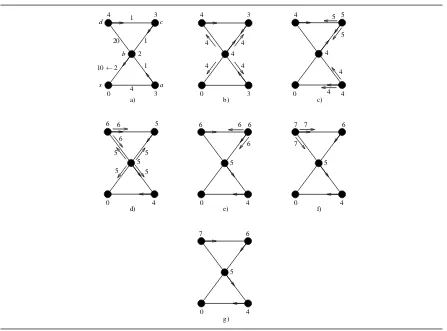
indicates that nodeyis the successor ofxtowards nodes. An arrowhead fromxtoyclose to edge(x,y)denotes that nodexis sending a message toycontaining the current distance fromstot, the value of such distance is reported close to the arrow.
4 1 3
1 1
4
c
a
20
3 0
2
b d
s
3 4
4 4 4
4 4
3 0
4 5
4 5 5
0 4
0 4
6
5 7
7 7
0 4
6 6
6 6
5 5
5 5
5 5
6 6
6 5
0 4
0 4
5
7 6
4
4 10←2
a) b) c)
d) e) f)
g)
Figure 3.Example of execution of DBF.
At a certain point in time, edge (b,s) changes its weight from 2 to 10 (see Figure 3(a)). When node b detects the weight increase, it updates the value of Db[b,s] to the minimum possible value, that is Db[b,s] =minu∈N(b){w(b,u) +Db[u,s]}=w(b,c) +Db[c,s] =4. Then, node bsends Db[b,s] to all its
neighbors (Figure 3(b)). As a consequence of such messages, nodes a and cupdate Da[b,s] and Dc[b,s],
respectively, compute their optimal distances tosthat are 4 and 5, respectively, and send them to their own neighbors (Figure3(c)). Nodessanddonly update Ds[b,s]and Dd[b,s], respectively. In Figure3(d), nodeb
updates Db[c,s]to 5 as a consequence of the message sent byc. Ascwas the successor node ofbtowardss,b
needs to update Db[b,s]to minu∈N(b){w(b,u) +Db[u,s]}=w(b,a) +Db[a,s] =5. After this update,bsends
Db[b,s]to its neighbors. Nodedbehaves similarly by updating its distance tosto 6. In Figures3(e)–3(g), the
message sent bybis propagated to nodescanddin order to update the distances from this nodes tos.
As a concluding remark of this section, we recall the reader that, if the nodes of the network are not synchronized, even in thestaticcase, i.e. when no change occurs in the network, it can be shown that the overall number of messages sent by DBF is, in the worst case, exponential with respect to the number of nodes in the network.
4. Diffuse Update Algorithm
This section describes the main characteristics of the Diffuse Update ALgorithm (DUAL) of [5]. The algorithm is described with respect to a sources∈V, and it starts every time a weight change ci ∈C =
4.1. Data Structures
DUAL is more complex than DBF, and uses different data structures in order to guarantee freedom from looping and counting to infinity phenomena. In detail, it stores, for each nodevand for each destinations, a slightly modified routing table where the two fields are theestimated distanceDv[v,s]and the so-calledfeasible
successorFSv[s], respectively. This latter value takes the place of the standard value of VIAv[s], and represents
an estimation onvia(v,s)that is always guaranteed to induce a loop-free VIAG[s](t)at any timet[5]. In order to
compute FSv[s], DUAL requires that each nodevbe able to determine, for each destinations, a set of neighbors
called the Feasible Successor Set, denoted as FSSv[s]. To this aim, each nodevexplicitly stores the topology
table, which contains, for eachu∈N(v), the distance Dv[u,s]fromutos. Then, it computes FSSv[s]by using the
SNCsufficient condition. In more details, nodeu∈N(v)is inserted in FSSv[s]if the estimated distance Dv[u,s]
fromutosis smaller than the so-calledfeasible distanceFDv[v,s]fromvtos. If a neighboru∈N(v), through
which the distance fromvtosis minimum, is in FSSv[s], thenuis chosen as feasible successor. Moreover, in
order to guarantee mutual exclusion in case multiple weight change operations occur, each nodevperforming DUAL uses some auxiliary data structures: (i) an auxiliary distance RDv[v,s], for eachs∈V; and (ii) a finite
state machine to process these multiple updates sequentially. The state of the machine consists, for eachs∈V, of three variables: the query origin flag Ov[s]and the state ACTIVEv[s], which contain an integer and a boolean
entry, respectively, and the replies status flag Rv[u,s], which contains a boolean entry for each neighboru∈N(v).
It follows that DUAL requiresΘ(n·maxdeg)space per node, as all the data structures stored by a nodevare arrays of sizen, with the exception of the topology table Dv[u,s]and the replies status flag, which are permanently
allocated and requireΘ(n·maxdeg)space. 4.2. Algorithm
The main core of DUAL is a sub-routine, named DIFFUSE-COMPUTATION, which is performed by a generic nodev, every time FSSv[s]does not include the nodeu∈N(v)through which the distance fromvto
sis minimum. The DIFFUSE-COMPUTATIONworks as follows: nodevsends queries to all its neighbors with its distance through FSv[s]by using message query. Accordingly,vsets Rv[u,s]to true, for each u∈N(v),
in order to keep trace of which neighbor has answered to thequerymessage (the value is set to false when a correspondingreplymessage is received). From this point onwardsvdoes not change its feasible successor tos until the DIFFUSE-COMPUTATIONterminates.
When a neighboru∈N(v)receives aquery, which triggers the execution of procedure QUERYwhose purpose is to try to determine if a feasible successor tos, after such update, exists. If so, it replies to thequeryby sending messagereplycontaining its own distance tos. Otherwise,upropagates the DIFFUSE-COMPUTATION toward the rest of the network. In details, it sends out queries and waits for the replies from its neighbors before replying tov’s originalquery. To guarantee that each node is involved in one DIFFUSE-COMPUTATION phase at the time, for a certains∈V, an appropriate finite state machine behaviour is implemented by variables Ov[s]and ACTIVEv[s]. Changes to distances, feasible distances and successors are allowed only under specific
circumstances. Moreover, an auxiliary variable RDv[v,s], representing an upper bound to Dv[v,s]is used by
each nodev, for eachs∈V, to answer to certain types of queries, under the same circumstances, in order to avoid loops. We refer the reader to [5] for an exhaustive discussion on the subject. In the same paper, the authors show that the DIFFUSE-COMPUTATIONalways terminates, i.e. that there exists, under the FIFOassumption, a time when a node receives messagesreplyby all its neighbors. At that point, it updates its distance and feasible successor, with the minimum value obtained by its neighbors and the neighbor that provides such distance. This is done during the execution of procedure REPLY, which is invoked upon the reception of each REPLYmessage. At the end of a DIFFUSE-COMPUTATIONexecution, a node sends messageupdatecontaining the new computed distance to its neighbors. As mentioned above, DUAL starts every time a nodexi detects a weight change
operationcioccurring on one of its adjacent edges, say(xi,yi). In what follows, the cases in whichciis a weight
decrease and a weight increase operation are considered separately.
Weight decrease.Ifciis a weight decrease operation on(xi,yi), nodexifirst tries to determine whether nodeyi
cican induce only decreases in the distances,SNCis trivially always satisfied by at least one neighbor, which is
either the current FSxi[s]oryiitself. This is done by invoking procedure DISTANCEDECREASE(yi,s)for all
s∈V, and the same routine is performed, symmetrically, by nodeyi. In any of the two cases, propagates the
change by sendingupdatemessages to its neighbors, with the aim of notifying either a change in the distance or in the distance and the feasible successor. Each node in the graph, which receives suchupdatemessage, in turn, determines whether FSv[s]has to be updated or not in the same way, and possibly propagates the change. Note
that, as the FIFOcase is under consideration, each node of the graph updates its data structures related tosat most once as a consequence ofci. Hence, since there are|σci,s|nodes that change their distance or feasible successor tosas a consequence ofciand since each nodevinσci,ssends at mostmaxdeg updatemessages, the number of messages, related to a sources, sent as a consequence of a weight decrease operationciisO(maxdeg· |σci,s|), while the number of steps required to converge isO(|σci,s|).
Weight increase.Ifciis a weight increase operation, the only nodes that sends messages, as a consequence of
operationciand w.r.t. a sources, are those inσci,sand their neighbors. In particular, aftercioccurs on(xi,yi), nodexitries, for eachs∈V, to determine whether a feasible successor still exists or not, by checking if nodes
in FSSv[s]still satisfySNC. This is done by inkoving procedure DISTANCEINCREASE(yi,s)for alls∈V. The
same routine is performed, symmetrically, by nodeyi. In the affirmative case, nodexiimmediately terminates its
computation and sends anupdatemessage to eachu∈N(xi)with the updated value of distance. Since we are
considering the FIFOcase, bySNCwe know that, in the above case, the path in VIAG[s]fromutosdoes not
containxi. Then, it follows that also nodeudoes not execute a DIFFUSE-COMPUTATIONnor sendupdatetoxi,
as a consequence ofci. In the negative case, i.e. nodexiperforms a DIFFUSE-COMPUTATION, and sensquery
messages to all its neighbors, and possibly (depending on the presence of alternative paths) induces other nodes in VIAG[s]to perform DIFFUSE-COMPUTATION. Whenxireceives all thereplymessages, it chooses as new
feasible successor a neighboru∈N(xi)which, in turn, does not perform DIFFUSE-COMPUTATIONnor send
updatemessages toxi, with respect tos, as a consequence ofci.
In any of the above cases, nodexisendsO(|N(xi)|)updatemessages while only in the second case, it
sendsO(|N(xi)|)querymessages and each of the nodes inN(xi)sendsO(1)replymessages. Note that each
nodev∈σci,sbehaves asxiwhen it receives eitherupdateorquerymessages from FSv[s]. As a consequence, it follows that the total number of messages sent by each nodev∈σci,sisO(|N(v)|) =O(maxdeg)and that the overall number of messages related to the sourcessent as a consequence of a weight increase operationciis
O(maxdeg· |σci,s|)while the number of steps required to converge isO(|σci,s|).
Since∑ki=1∑s∈V|σci,s|=∆, it follows that the overall number of messages sent by DUAL during a sequence of weight modificationsC = (c1,c2, ...,ck), in the FIFOcase, and for each possible sources, is given
by∑ki=1∑s∈VO(maxdeg· |σci,s|) =O(maxdeg·∆), while the overall number of steps required by the algorithm to converge is∑ki=1∑s∈VO(|σci,s|) =O(∆). By the above discussion the next theorem follows.
Theorem 4([5]). DUALrequires O(maxdeg·∆)messages, O(∆)steps, andΘ(n·maxdeg)space occupancy per node.
4.3. Example of Execution
Q Q Q Q 12 11 4 0 10 12 11 4 0 5 7 6 4 0 5
g) h) i)
11 4 0 10 12 11 4 0 10 12 11 4 0 10
d) e) f)
4 3 3 0 2 4 3 3 0 10 4 11 4 0 10
a) b) c)
1
1 1
4 20
10←2
c a s d b Q Q Q R(4) R(0) 12 R(4) Q R(10) R(11) R(12) Q R(10) R(11) U U U U
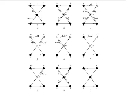
Figure 4.Example of execution of DUAL.
b’squery, it simply sends areplybecause it has a feasible successor. However, it becomes involved in the DIFFUSE-COMPUTATIONwhen it receives thequeryfrom nodec(Figure4(d)). When nodedreceives all the replies to itsquery(Figure4(e)), it computes its new distance and successor (12 andc, respectively), and sends a replytoc’squery(Figure4(f)). Nodescandboperate in a similar manner when they receives all the replies to their respective queries (Figure4(f)–4(g)). At this point, the DIFFUSE-COMPUTATIONis terminated and nodeb sends messagesupdatecontaining the new computed distance to notify it to its neighbors (Figure4(h)). Such messages are propagated to the entire network in order to update the distances according to paths tosinduced by successors nodes (Figure4(i)).
As a final observation, notice that, the undesirable count-to-infinity phenomenon shown in Figure2of Section3, induced by the use of DBF, does not occur if DUAL is used, withSNC. In fact, for instance, at step 2, theSNCprevents nodevto choosebas its successor, since the loop-free test fails. This triggers an execution of DIFFUSE-COMPUTATION, which is guaranteed to always produce an acyclic sub-graph induced by the feasible successors [5].
5. Loop Free Routing Algorithm
This section describes the Loop Free Routing (LFR) algorithm, introduced for the first time in [39], and then extended and established in [29]. The algorithm consists of four procedures named UPDATE, DECREASE, INCREASEand SENDFEASIBLEDIST, respectively. The algorithm is described with respect to a sources∈V, and it starts every time a weight changeci∈C = (c1,c2, ...,ck)occurs on an edge(xi,yi).
5.1. Data Structures
table, that consists of two arrays Dv[v,s]and FSv[s], that store theestimated distanceand the so-calledfeasible
via, respectively. This latter value represents a different kind of estimation onvia(v,s)that is always guaranteed to induce loop-free VIAG[s](t)at any timet[29]. In addition, for eachs∈V, a nodevexecuting LFR stores
the following data structures: STATEv[s]: the state of nodevwith respect to sources(vis inactivestate and
STATEv[s] =trueif and only if it is performing procedure INCREASEor procedure SENDFEASIBLEDISTwith
respect tos); UDv[s]: the estimated distance fromvtosthrough the current FSv[s](in particular, ifvis active
UDv[s] is always greater than or equal to Dv[v,s], otherwise they coincide). In addition, to implement the
topology table and thus SNC, a node vstores atemporarydata structure TEMPDv. Such array TEMPDv is
allocated atvfor a certainsonly when needed, that is whenvbecomes active with respect to a certains, and it is deallocated right aftervturns back in passive state with respect to the sames. The entryTEMPDv[u][s]contains
UDu[s], for eachu∈N(v), and henceTEMPDvtakesO(maxdeg)space per node.
5.2. Algorithm
At any timet<t1, before LFR starts, it is assumed that, for each pair of nodesv,s∈V, the values stored in Dv[v,s](t)and FSv[s](t)are correct, that is Dv[v,s](t) =dt(v,s)and FSv[s](t)∈viat(v,s). The description
focuses on a distinguished nodes∈Vand each nodev∈V, at timet, is assumed to be passive with respect tos. The algorithm starts when the weight of an edge(xi,yi)changes. As a consequence,xi(yi, respectively)
sends toyi(xi, respectively) messageupdate(xi,s, Dxi[xi,s])(update(yi,s, Dyi[yi,s]), respectively). Messages received at a node are stored in a queue and processed in FIFO order to guarantee mutual exclusion. If an arbitrary nodevreceivesupdate(u,s, Du[u,s])fromu∈N(v), then it performs procedure UPDATE, which simply
compares Dv[v,s]with Du[u,s] +w(u,v)to determine whethervneeds to update its estimated distance and or its
estimated feasible via tos.
If node vis active, then the processing of the message is postponed by enqueueing it into the FIFO queue associated tos. Otherwise, we distinguish three cases, and discuss them separately, depending on the type of change in the estimated distance (or feasible via) that is induced by the message. In particular, if Dv[v,s]>Du[u,s] +w(u,v), thenvperforms procedure DECREASE, while if Dv[v,s]<Du[u,s] +w(u,v), then
vperforms procedure INCREASE. Finally, if nodevis passive and Dv[v,s] =Du[u,s] +w(u,v)then it follows
that there is more than one shortest path fromvtos. In this case the message is discarded and the procedure ends. Weight decrease.When a nodevperforms procedure DECREASE, it simply updatesD,UDandFSdata structures by using the updated information provided byu. Then, the update is forwarded to all neighbors ofvwith the exception of FSv[s]which is nodeu.
Weight increase. When a nodevperforms procedure INCREASE, it first checks whether the update has been received from FSv[s]or not. In the negative case, the message is simply discarded while, in the affirmative
case (only)vneeds to change its estimation on distance and feasible via tos. To this aim, nodevbecomes active, allocates the temporary data structureTEMPDv, and sets UDv[s]to the current distance through FSv[s].
At this point,vfirst performs the so called LOCAL-COMPUTATION, which involves all the neighbors ofv. If the LOCAL-COMPUTATIONdoes not succeed, then nodevinitiates the so called GLOBAL-COMPUTATION, which involves in the worst case all the other nodes of the network.
During the LOCAL-COMPUTATION, nodevsendsget.distmessages, carrying UDv[s], to all its neighbors,
with the exception ofu. A neighbork∈N(v)that receives aget.distmessage, immediately replies with the value UDk[s], and ifkis active, it updatesTEMPDk[v][s]to UDv[s]. When nodevreceives these values from its
neighbors, it stores them in the arrayTEMPDv, and it uses them to compute the minimum estimated distance
Dmintosand the neighbor VIAminwhich gives such a distance.
At the end of the LOCAL-COMPUTATIONvchecks whether a feasible via exists, by executing the loop-free test, according to theSNC. If the test fails, thenvinitiates the GLOBAL-COMPUTATION, in which it entrusts the neighbors the task of finding a loop-free path. In this phase,vsendsget.f easible.dist(v,s, UDv[s])message to
to compute the minimum estimated distance Dmintosand the neighbor VIAminwhich gives such a distance.
At this point,vhas surely found a feasible via tosand hence it deallocatesTEMPDv, updates Dv[v,s], UDv[s]
and FSv[s]and propagates the change by sendingupdatemessages to all its neighbors. Finally,vturns back in
passive state and starts processing another message in the queue, if any.
A nodek∈N(v)that receives aget.f easible.distmessage performs procedure SENDFEASIBLEDIST. If FSk[s] =vandkis passive, then procedure SENDFEASIBLEDISTbehaves similarly to procedure INCREASE.
The only difference is that SENDFEASIBLEDISTneeds to answer to theget.f easible.distmessage. However, within SENDFEASIBLEDIST, the LOCAL-COMPUTATIONand the GLOBAL-COMPUTATIONare performed with the aim of sending a reply with an estimated loop-free distance in addition to that of updating the routing table. In particular, nodekneeds to provide tova new loop-free distance. To this aim, it becomes active, allocates the temporary data structureTEMPDk, and sets UDk[s]to the current distance through FSv[s]. Then, as in
procedure INCREASE,kfirst performs the LOCAL-COMPUTATION, which involves all the neighbors ofk. If the LOCAL-COMPUTATIONfails, that isSNCis violated, then nodekinitiates the GLOBAL-COMPUTATION, which involves in the worst case all nodes of the network. At this pointkhas surely found an estimated distance to swhich is guaranteed to be loop-free and hence, differently from INCREASE, it sends this value to its current viavas answer to the get.f easible.dist message. Now, as in procedure INCREASE, node kcan deallocate TEMPDv, update its local data structures Dv[v,s], UDv[s] and FSv[s], and propagate the change by sending
updatemessages to all its neighbors. Finally,vturns back in passive state and starts processing another message in the queue, if any.
Concerning the space complexity, LFR takesO(n+maxdeg·δ)space per node, as all the data structures, stored by a nodev, are arrays of sizen, with the exception ofTEMPDv[·][s]which is allocated only when nodev
becomes active for a certain destinations, that is only ifv∈δci,s, and deallocated whenvturns back in passive state fors, that is at mostδ times. As each entryTEMPDv[·][s]requiresO(maxdeg)space, the total space per
node isO(n+maxdeg·δ)in the worst case.
Concerning the message and time complexity, given a sourcesand a weight change operationci∈C on
edge(xi,yi), the cases in whichciis a weight decrease or a weight increase operation are considered separately.
Ifciis a weight decrease operation, only nodes inσci,supdate their data structures and send messages to their neighbors. In detail, a nodevcan update its data structures related tosat most once as a consequence ofciand,
in this case, it sends|N(v)|messages. Hence,vsends at mostmaxdegmessages. Since there are|σci,s|nodes that change their distance or via tosas a consequence ofci, the number of messages related to the sourcessent
as a consequence of a weight decrease operationciisO(maxdeg· |σci,s|), while the number of steps required to converge isO(|σci,s|).
Ifciis a weight increase operation, the only nodes which send messages with respect to operationciand
sourcesare those inσci,sand the neighbors of such nodes. In detail, each time that a nodev∈σci,sexecutes procedures INCREASEand SENDFEASIBLEDIST, it sendsO(|N(v)|)messages and each of the nodes inN(v) sendsO(1)messages, for a total number ofO(|N(v)|) =O(maxdeg)messages sent. In the FIFOcase, nodev performs either procedure INCREASEor procedure SENDFEASIBLEDISTat most once with respect tociands. It
follows that eachv∈σci,ssends at mostO(maxdeg)messages. Therefore, the overall number of messages related to the sourcessent as a consequence of operationciisO(maxdeg· |σci,s|)while the number of steps required to converge isO(|σci,s|). Now, since∑
k
i=1∑s∈V|σci,s|=∆, it follows that the overall number of messages sent during the whole sequenceC and for each possible sources, is given by∑ki=1∑s∈VO(maxdeg· |σci,s|) =O(maxdeg·∆), while the overall number of steps required by the algorithm to converge is∑ki=1∑s∈VO(|σci,s|) =O(∆).
The next theorem follows from the above discussion.
Theorem 5([29]). LFRrequires O(maxdeg·∆)messages, O(∆)steps, and O(n+maxdeg·δ)space occupancy per node.
5.3. Example of Execution
(2,2) (4,4) (3,3) (3,3) (0,0) (2,2) (4,4) (3,3) (3,3) (0,0) (4,4) (3,3) (3,3) (0,0) (2,10) (2,10) (4,4) (3,11) (3,11) (0,0)
2→10
u(0) c a s d b c a s d b 4 3 c a s d b 20 1 1 4 c a s d b 1 3 gF(10) gF(10) c a s d b 4 c a s d c a s c a s d b c a s d c a s d
(a) (b) (c) (d)
(e) (f) (g) (h)
(i) 4 0 4 (j) (k) u(2) gF(11) b b b b 10 10 d gD(12) gD(10) gD(10) gD(11) gD(11) (2,10) (4,12) (0,0) (3,11) c a s d b (4,4) (2,10) (0,0) (3,11) (4,12) (4.4) (2,10) (0,0) (12,12) (3,11) (0,0) (2,10) 11 u(11) (11,11) (12,12) u(12) u(4) (4,4) (4,4) (5,5) (0,0) (12,12) (11,11) (4,4) u(5) u(5) (0,0) (4,4) (5,5) (6,6) u(6) (12,12) (5,5) (4,4) (0,0) (7,7) (6,6) gD(10) gF(10) gF(12) 12 u(7) u(5) u(5)
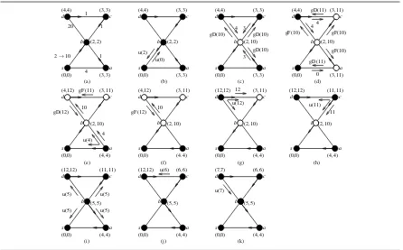
Figure 5.Example of execution of LFR.
and UDv[s]by a pair of values associated tov. Before LFR starts it is assumed that all nodes are inpassivestate,
that is none of them is involved in a computation with respect tos. Passive nodes are represented as black circles, while active nodes by white circles. In the example, the algorithm starts when the weight of(b,s)increases from 2 to 10 (Figure5(a)). As a consequencebsends tosmessageupdate(b,s, Db[b,s]), andssends tobmessage update(s,s, Ds[s,s]), denoted as u(2) and u(0), respectively (Figure5(b)).
When a nodevreceives anupdatemessage with an increased distance tos, it checks whether it comes from FSv[s]and, in the affirmative case, it performs Procedure INCREASE, otherwise it discards the message.
Hence, whensreceives u(2), it immediately discards it and terminates, as FSs[s]6=b. On the other hand, when
nodeb, receives u(0), since FSb[s] =sand Db[b,s]<Ds[s,s] +w(b,s), it needs to update its own routing table
and hence it performs Procedure INCREASE. In detail,bfirst performs the LOCAL-COMPUTATIONin which it tries to understand whether its routing table can be updated by using only the distances tosof its neighbors. To this aim,b switches to theactivestate, sets TEMPDb[s][s] =0 and UDb[s] =TEMPDb[s][s] +w(b,s) = 0+10=10, and it sends to all its neighbors, except FSb[s] =s, aget.distmessage carrying UDb[s]denoted as
gD(10) (Figure5(c)). When a nodek∈N(b)receives gD(10), it immediately replies tobby sending UDk[s]
(Figure5(c)). By using the replies of its neighbors,bcomputes Dmin =min{TEMPDb[k][s] +w(b,k)|k∈N(b)}
and VIAmin=argmin{TEMPDb[k][s] +w(b,k)|k∈N(b)}and performs the loop-free test of theSNC, to check
whether the provided distance corresponds to a loop-free path or not. ThenbcomparesTEMPDb[VIAmin][s]with
Db[b,s], which represents the last value of a loop-free distance computed byb. If the test succeeds, it follows
thatbhas a feasible via tos. Then it turns back in passive state, updates its routing table and propagates the change to its neighbors. Otherwise,bperforms the GLOBAL-COMPUTATION, where it computes a loop-free path by involving the other nodes of the graph. In this phasebsends to its neighbors aget.f easible.distmessage (denoted as gF in the figure), bringing the most up to date estimated distance tosthrough the current successor FSb[s]ofb. In this case, Dmin =Da[a,s] +w(b,a) =4 andTEMPDb[a][s] =3>Db[b,s] =2, hencebperforms
GLOBAL-COMPUTATION(Fig.5(d)).
When a neighbor k ofb receives get.f easible.dist, it performs Procedure SENDFEASIBLEDIST. In detail,kfirst checks whether FSk[s]6=bor STATEk[s] =true. In this case,kimmediately replies tobwith
UDk[s] =TEMPDb[b][s] +w(b,k)(for example nodeasets UDa[s] =10+1=11 in Figure5(d)), performs
first LOCAL-COMPUTATION and then GLOBAL-COMPUTATION(nodesa andcin Figures5(d)–5(f)), in a way similar to Procedure INCREASE. To this aim, nodea performs LOCAL-COMPUTATION(Figure 5(d)), which succeeds since TEMPDa[s][s] =0, and replies to b with 4 (Figure 5(e)). Differently from a, the
LOCAL-COMPUTATIONof nodecfails, and hencecperforms GLOBAL-COMPUTATIONas well, by sending gF(11) tod(Fig.5(e)). When nodedreceives such message, it performs LOCAL-COMPUTATIONby sending gD(12) tobwhich replies with UDb[s] =106=Db[b,s] =2. Since theSNCis not satisfied atd, because
• min{TEMPDd[z][s] +w(d,z)|z∈N(d)}=12
• argmin{TEMPDd[z][s] +w(d,z)|z∈N(d)}=cand
• TEMPDd[c][s] =11>Dd[d,s] =4
thend performs GLOBAL-COMPUTATION by sending gF(12) tob, which immediately replies with 10, and updatesTEMPDb[d][s] =12 (Fig.5(f)).
At the end of this process, nodedfinds a new feasible via, nodec, and replies tocwith the corresponding minimum estimated distance Dc[c,s] +w(d,c) =12. In addition, nodedupdates its routing table and propagates
the change to its neighbors. Whencreceives the answer to the gF message fromd(Figure5(g)) it behaves asd, by sending Db[b,s] +w(b,c) =11 tob, updating its routing table and propagating the change to its neighbors.
Whenbreceives all the replies to its gF messages (Fig.5(h)), it is able to compute the new loop-free shortest path tos, to update UDb[s] =Db[b,s] =5, to turn back in passive state and to propagate the change by means of
updatemessages (Fig.5(i)). Theupdatemessages induce the neighbors ofbto update their routing tables as described above forb. As the value UDb[s], sent bybduring the GLOBAL-COMPUTATIONis an upper bound to
Db[b,s], theseupdatemessages induce the neighbors to perform procedure DECREASE(Figure5(j–k)).
As a final observation of the section, notice that, the undesirable count-to-infinity phenomenon shown in Figure2of Section3, induced by the use of DBF, does not occur if LFR is used, withSNC, as well as for DUAL. In fact, for instance, at step 2, theSNCprevents nodevto choosebas its successor, since the loop-free test fails after the LOCAL-COMPUTATIONphase. This triggers an execution of GLOBAL-COMPUTATION, which is guaranteed to always produce an acyclic sub-graph induced by the feasible successors [29].
6. Distributed Computation Pruning
This section describes the Distributed Computation Pruning (DCP) technique, introduced for the first time in [40] and then extended in [30]. The approach is not an algorithm by itself. Instead, it is a general technique that can be applied on top of a Distance-Vector algorithm for distributed shortest paths with the aim of improving its performance. Given a generic Distance-Vector algorithmA, the combination of DCP withAinduces a new algorithm, denoted byA-DCP. The DCP technique is designed to be efficient mainly in power-law networks, by forcing the distributed computation to be carried out only by a subset of few nodes of the network.
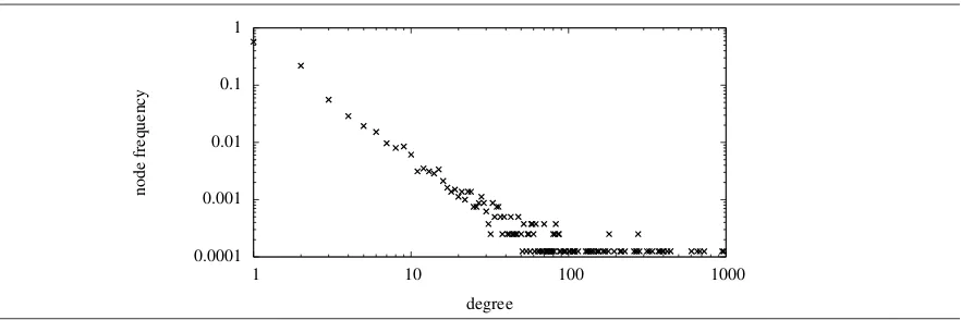
6.1. Power-law Networks
Apower-law network, in the most general meaning, is a network where the distribution of the nodes’ degree follows a power-law trend, thus having many nodes with low degree and few (core) nodes with very high degree (see e.g. [32]). Such class of networks is very important from the practical point of view, since it includes many of the currently implemented communication infrastructures, like the Internet, the World Wide Web, some social networks, and so on. For this reason, a number of methods to generate artificial topologies exhibiting a power-law behaviour have been proposed in the literature. Among them, the most prominent are the Barabási-Albertmodel [32] and the Generalized Linear Preference (GLP) model [33].
centralifviis central, for each 0≤i≤j. Any edge belonging to a central path is calledcentral edge. A path
P={v0,v1,. . .,vj}ofGisperipheralifv0is central,vj is peripheral, and allvi, for each 1≤i≤j−1, are
semi-peripheral. In this case,v0is called theownerofPand of any node belonging toP. Any edge belonging to a peripheral path, accordingly, is calledperipheral edge. Finally, a pathP={v0,v1,. . .,vj}ofGissemi-peripheral
ifv0andvjare two distinct central nodes, and allviare semi-peripheral nodes, for each 1≤i≤j−1. Nodesv0 andvjare called thesemi-ownersofPand of any node belonging toP. Any edge belonging to a semi-peripheral
path is called semi-peripheral edge. A further distinction for semi-peripheral paths occurs ifv0≡vj. In this case
Pis called asemi-peripheral cycle, and nodev0≡vjis called thecycle-ownerofPand of any node belonging to
P. Each edge belonging to such a path is calledcyclic edgeand each nodeu6=v0inPis calledcyclic node. DCP has been designed to exploit the aforementioned topological properties of power-law networks in order to reduce the communication overhead induced by distributed computations executed by Distance-Vector algorithms. In particular, it forces the distributed computation to be carried out by the central nodes only (which are few in power-law networks). Non-central nodes, which are instead the great majority, play a passive role and receive updates about routing information from the respective owners, without taking part to any kind of distributed computation and by performing few trivial operation to update their routing data. Hence, it is clear that the larger is the set of non-central nodes of the network, the bigger is the improvement in the pruning of the distributed computation and, consequently, in the global number of messages sent byA-DCP.
6.2. Data Structures
In order to be implemented, DCP requires a generic node ofGto store some additional information with respect to those required byA. In particular, each nodevneeds to store and update information about adjacent non-central paths ofG. To this aim,vmaintains a data structure called CHAINPATH, denoted as CHPv, which is
an array containing one entry CHPv[s], for each central nodes. CHPv[s]stores the list of all edges, along with
their weights, belonging to those non-central paths that contains. To build the CHAINPATHdata structure, it is assumed thatvknows the degree of all nodes of the network belonging to non-central paths. The following properties clearly hold: i) a central node obviously does not appear in any list of CHPv; ii) a peripheral node
appears in exactly one list CHPv[s], wheres∈V is its owner; iii) a semi-peripheral node appears in exactly two
lists CHPv[v0]and CHPv[vj−1], if it belongs to a semi-peripheral path (v0andvj−1are its semi-owners), while it appears in a single list CHPv[v0], if it belongs to a semi-peripheral cycle (v0is its cycle-owner). Hence, a node v, by using CHPvis able to determine locally its type, and, in the case it is not central, it is also able to compute
its owner, semi-owners, or cycle-owner. As shown in [30], the worst case space occupancy overhead per node due to the use of CHAINPATHisO(n).
6.3. Description
The behaviour of a generic algorithmA, when combined with DCP, can be summarized as follows. The main difference resides in the fact that in a classic routing algorithm every node performs the same code thus having the same behaviour, while inA-DCP, given the nodes’ and edges’ classification, central and non-central nodes are forced to have different behaviours. In particular, central nodes detect (and handle) changes concerning all kinds of edges, while peripheral, semi-peripheral, and cyclic nodes detect (and handle) changes concerning only peripheral, semi-peripheral, and cyclic edges, respectively. In what follows, we summarize how each of the possible changes is handled byA-DCP.
of the path. Thesp.querymessage contains only one field, i.e. the objectsof the computation that has originated the message. When a semi-peripheral node receives asp.query(s)message from one of its two neighbors j, it simply performs a store-and-forward step and sends asp.query(s)message to the other neighbork6= j. The store-and-forward step is performed in a way that the ordering of the messages is preserved. A central node rthat receives asp.query(s)message from one of its semi-peripheral neighborsu, simply replies touwith a sp.reply(s, Dr[r,s])message, which carries the estimated distance ofrtowardss, which was requested byx(y,
respectively). When a semi-peripheral node receives asp.reply(s, Dr[r,s])message from one of its two neighbors
j, it simply performs a store-and-forward step and sends asp.reply(s, Dr[r,s])message to the other neighbor
k6= j. The strategy terminates whenever the central nodex(y, respectively) receivessp.reply(s, Dr[r,s]): upon
that event,x(y, respectively) stores Dr[r,s]and uses it, if needed, while executing the routine provided byAfor
the distributed computation of shortest paths.
Oncex(y, respectively) has updated its own routing data toward a certain central nodes, it propagates the variation to all its neighbors through agen.update(s, Dx[x,s])(gen.update(s, Dy[y,s]), respectively), which
carries an updated value of Dx[x,s](Dy[y,s], respectively). When a generic nodevreceives agen.updatemessage
from a neighboru, it executes a procedure, called GENERALIZEDUPDATE, which, as first step, stores the current value of Dv[v,s]in a temporary variable Doldv [s]. Then, according to its status, the node performs different steps,
which can be summarized as follows. Ifvis central, then it handles the change and updates its routing information toward the central nodesby using the proper procedure ofA, i.e. HANDLEUPDATE, HANDLEINCREASE, or HANDLEDECREASE, depending on the original structure ofA, and forwards the change through the network accordingly.
If, instead,vis a peripheral node whose owner is noder, then Dv[v,s] is trivially updated by setting
Dv[v,s] =Dv[v,r] +Dv[r,s]. Moreover, any specific data structure ofAis accordingly updated, and Dv[r,s]
is propagated to the other neighbor ofv. Moreover, ifvis a cyclic node whose cycle-owner is noder, thenv sets Dv[v,s] =Dv[v,r] +Dv[r,s]. Moreover, since Dv[r,s]is not changed, any specific data structure ofAis
accordingly updated, and Dv[r,s]is propagated to the other neighbor ofv.
Finally, ifvis a semi-peripheral node whose semi-owners are nodesr1andr2, then the message carries the estimated distance from eitherr1orr2toswhich can be used to update distances. In details, let us assume that the message carries Dr1[r1,s], the other case is symmetric. Letuandzbe the neighbors ofvwhich are closer (in terms of number of edges) tor1andr2, respectively. If the distance fromvtosis not affected by the change of Dr1[r1,s], that is Dr1[r1,s]increases but VIAv[s]6=u, thenvsimply discards the message. Otherwise, two cases may arise:
• (i) if Dr1[r1,s] is increased and VIAv[s] =u, then nodevupdate Dv[v,s]as the weight of the shortest between two paths: that formed by the shortest path fromr1tosplus the path fromr1tov, and that formed by the shortest path fromztosplus edge(z,v);
• (ii) if Dr1[r1,s]is decreased enough to induce a decrease also to Dv[v,s], thenvupdates Dv[v,s]as the weight of the path formed by the shortest path fromr1tosplus the unique path fromr1tov.
In both the above mentioned cases, any specific data structure ofAis updated accordingly, and Dr1[r1,s]is propagated toz. This behaviour mimics the distributed Bellman-Ford algorithm equipped with the split horizon heuristic [41, Section 6.6.3]: the information about the route for a particular node is never sent back in the direction from which it was received.
After updating the routing information toward the central node s, v calls a procedure called PERIPHERYUPDATE, usingsand Doldv [s]as parameters. This routine first verifies whether the routing table entry ofsis changed or not and, in the affirmative case, it updates the routing information about the non-central nodes whose owner, semi-owner, or cycle-owner iss, if they exist, as follows:
• for each peripheral nodezwhose owner iss, nodevsets Dv[v,z]equal to the weight of the unique path
fromstozplus the weight of the shortest path fromvtos.
• for each cyclic nodezwhose cycle-owner iss, nodevsets Dv[v,z]equal to weight of the shortest between
• for each semi-peripheral nodezsuch that one of the semi-owner nodes iss, nodevperforms procedure INNERSEMIPERIPHERYUPDATE, if z and v lie on the same semi-peripheral path, and procedure OUTERSEMIPERIPHERYUPDATE, otherwise. These procedures update the routing information towardz by exploiting the data stored in the CHAINPATH. In detail, procedure INNERSEMIPERIPHERYUPDATE updates Dv[v,y]by comparing the weight of the only two paths that connectvandz. Note that, such two
paths include the shortest paths between the semi-owners ofvandvitself.
In particular, ifSis the semi-peripheral path that includesvandzwhose semi-owners arer1andr2, nodev computes the weight D1of the unique sub-path ofSfromvtoz, and determines the neighbor VIA1ofv that belongs to such sub-path. Then, ifvbelongs to the sub-path ofSthat connectsztor1(this detail can easily be deduced from the CHAINPATH), it computes the weight D2of the path formed by the sub-path ofSfromztor2plus the shortest path fromvtor2. Note that such shortest path might contain noder1. Otherwise, nodevcomputes the weight D2of the path formed by the sub-path ofSfromztor1plus the shortest path fromvtor1. Finally, nodevsets Dv[v,z]to the minimum weight of the above two possible
paths and, accordingly, it updates VIAv[z].
Similarly, procedure OUTERSEMIPERIPHERYUPDATEupdates Dv[v,z]by comparing the weight of the
only two paths that connectvandz. Note that such paths include the shortest paths between the semi-owners ofzandv. In detail, ifSis the semi-peripheral path that containszandr1andr2are the semi-owners ofS, nodevfirst computes two values Dr1and Dr2, equal to the weight of the path formed by the path betweenzandr1(zandr2, respectively) plus the shortest path betweenvandr1(vandr2, respectively), then sets Dv[v,z]equal to the minimum of the weights of these two possible paths and, accordingly, it
updates VIAv[z].
Case (ii). If a weight change occurs on a peripheral edge (x,y1), belonging to a peripheral path P=
{r,. . .,x,y1,. . .,yn} whose owner is r, then node x (y1, respectively), handles the change by sending a peri.change(x,y1,w(x,y1)) message to each of its neighbors. In this case, the distance from each node of the network toxdoes not change, except for those nodesypwithp=1,. . .,n(which are topologically further
thanxfromr). Each of these nodes, after receiving theperi.change(x,y1,w(x,y1))message, first updates the CHP with the new value ofw(x,y1)and then computes the distance toxand to all the other nodessof the network by simply adding to Dyp[yp,s]the weight change on edge(x,y1).
When a generic nodev, different from nodesyp, receives messageperi.change(x,y1,w(x,y1)), it first verifies whether the update has been already processed or not, by comparing the new value ofw(x,y1)with the one stored in its CHP. In the first case the message is discarded. Otherwise, it updates its CHP with the updated valuew(x,y1)and its routing information only toward nodesyp, as the shortest path towardxdoes not
change. In particular, nodevsets Dv[v,yp] =Dv[v,r] +Dv[r,yp], where Dv[r,yp]is the weight of the peripheral
path fromrtoyp(note that, for eachv∈P,v6=yp, Dv[v,yp]is computed by using only the information stored
inside the CHP because it is equal to the weight of the peripheral path fromvtoyp). Then, it propagates
peri.change(x,y1,w(x,y1))over the network by a flooding algorithm.
Case (iii).If the weight of a semi-peripheral edge(x,y), whose semi-owner nodes arer1andr2, changes, then nodex(y, respectively) sends two kinds of messages: asemi.change(x,y,w(x,y)), to each of its neighbors, and agen.update(s, D·[·,s]tox(y, respectively), for each central nodessuch that VIAx[s]6=y(VIAy[s]6=x,
When a generic nodevreceives agen.update(s, D·[·,s]message from a neighboru, it executes procedure GENERALIZEDUPDATE(s, D·[·,s]. After updating the routing information toward a central nodes, nodevcalls the procedure PERIPHERYUPDATEusingsand Doldv [s]as parameters. The procedure works as in the case of a central edge weight change (see Case (i)).
Case (iv). If the weight of a cyclic edge(x,y)changes, both nodesxandysend acycl.change(x,y,w(x,y)) message to each of their neighbors. Letrbe the cycle-owner node of bothxandy. When a generic nodev receives messagecycl.change, it first verifies whether the update has been already processed or not, by comparing the new value ofw(x,y)with the one stored in its CHP. In the first case the message is discarded. Otherwise, nodevfirst updates its CHP with the updated value ofw(x,y)and propagatescycl.change(x,y,w(x,y))over the network by a flooding algorithm. Then, two cases can occur: either nodevbelongs to the same semi-peripheral cycle ofxandyor not.
• In the first case, nodevfirst computesdα=D
v[v,s]−Dv[v,r]and, hence, updates the routing information
toward all the nodes of the semi-peripheral cycle, includingr, by using the CHP data structure. Then, if Dv[v,r]changes, it updates the routing information toward all the other central nodessof the network by
setting Dv[v,s] =Dv[v,r] +dα. After updating the routing information toward a central nodes, nodev
calls the procedure PERIPHERYUPDATEusingsand Doldv [s]as parameters. The procedure works as in the case of a central edge weight change (see Case (i)).
• In the second case,vcomputes, for each nodezof the semi-peripheral cycle, the shortest path distance betweenzand its cycle-owner noderby using the CHP data structure. Finally, it assigns Dv[v,z] =
Dv[v,r] +Dv[r,z].
6.4. CombiningDCPwithDUAL
This section describes the combination of DCP to DUAL, denoted as DUAL-DCP. The main changes deriving by the application of DCP to DUAL can be summarized as follows.
On the one hand, if the weight of a central edge(u,v)changes, then nodevverifies, only with respect to each central nodes, whether Dv[v,s]>Dv[u,s] +w(u,v)or not (note that the behaviour of nodeuis symmetric with
respect to the weight change operation). In the first case, nodevsets Dv[v,s] =Dv[u,s] +w(u,v)and FSv[s] =u
and propagates the change to all its neighbors. In the second case, nodevfirst checks whether FSv[s] =uor not.
If FSv[s]6=u, the node terminates the update procedure. Otherwise, nodevtries to compute a new FSv[s]. In this
phase, if no neighbor ofvsatisfiesSNCand nodevneeds to perform the DIFFUSE-COMPUTATION, it sends out querymessages only to its central neighbors. Moreover, with the aim of knowing the estimated distance of each of the semi-owner of the semi-peripheral paths which nodevbelongs to, nodevperforms theTRAVERSE-PATH phase and sendssp.querymessages to each of its semi-peripheral neighbors. When nodevreceives all the replies to these messages, it updates its routing information towardssand propagates the change to all its neighbors. In all the cases, if the distance towardsschanges, nodevis able to update its routing information towards all the nodes in the non-central paths ofs, if they exists.
On the other hand, if a weight change occurs on either a peripheral or a cyclic edge, then the nodes adjacent to the edge behave as described in Section6. The only difference with respect to the generic case is that involved nodes also update their topology table. Finally, if a weight change occurs on a semi-peripheral edge, differently from the general case, semi-peripheral nodes do not need to ask information to their neighbors, as DUAL permanently stores the topology table.
6.5. CombiningDCPwithLFR
This section describes the combination of DCP to LFR, denoted as LFR-DCP. The main changes deriving by the application of DCP to LFR can be summarized as follows.
If the weight of a central edge(u,v)changes, then nodevverifies, only with respect to central nodes s∈Vc, whether Dv[v,s]>Dv[u,s] +w(u,v)or not (note that the behaviour of nodeuis symmetric with respect
to the weight change operation). In the first case, nodevsets Dv[v,s] =Dv[u,s] +w(u,v)and FSv[s] =uand
FSv[s]6=u, the node terminates the update procedure. Otherwise, nodevperforms LOCAL-COMPUTATION, by
sendingget.distmessage to all its neighbors. If the LOCAL-COMPUTATIONsucceeds, nodevupdates its routing information and propagates the change. Otherwise, nodevneeds to perform the GLOBAL-COMPUTATIONand it sends outget.f easible.distmessages only to its central neighbors. Moreover, with the aim of knowing the estimated distance of each of the semi-owner of the semi-peripheral paths which nodevbelongs to, nodev performs theTRAVERSE-PATHphase and sendssp.querymessages to each of its semi-peripheral neighbors. When nodevreceives all the replies to these messages, it updates its routing information towardssand propagates the change to all its neighbors. In all the cases, if the distance toschanges, nodevis able to update its routing information towards all nodes in the non-central paths ofs, if they exists. If a weight change occurs on a peripheral, semi-peripheral or a cyclic edge, then the nodes adjacent to the edge behave as described in Section6.
6.6. Practical Effectiveness ofDCP
This section describes the results of the experimental study proposed in [30], which considers algorithms DUAL, LFR, DUAL-DCP and LFR-DCP, and shows the practical effectiveness of the use of DCP. Experiments have been performed both on real-world and artificial instances of the problem, subject to randomly generated sequences of updates. In detail, both the power-law networks of theCAIDA IPv4 topology dataset[31], and the random power-law networks generated by theBarabási-Albertalgorithm [32] were used. In particular, simulations have been ran on a CAIDA instance with 8000 nodes and 11141 edges, namedGIP−8000, and on a Barabási–Albert instance with 8000 nodes and 12335 edges, namedGBA−8000.GIP−8000has average node degree equal to 2.8, a percentage of degree 1 nodes approximately equal to 38.5%, and a percentage of degree 2 nodes approximately equal to 33%;GBA−8000has average node degree equal to 3.1, a percentage of degree 1 nodes approximately equal to 45%, and a percentage of degree 2 nodes approximately equal to 26%.
The experimental results provided in the considered paper have shown that the combinations of both DUAL and LFR with DCP provide a huge improvement in the global number of messages sent onGIP−8000. In particular, the ratio between the number of messages sent by DUAL-DCP and those sent by DUAL is within 0.03 and 0.16 which means that DUAL-DCP sends a number of messages which is between 3% and 16% that of DUAL. The ratio between the number of messages sent by LFR-DCP and those sent by LFR is within 0.10 and 0.26.
Similar results are obtained onGBA−8000. In more details, the ratio between the number of messages sent by DUAL-DCP and those sent by DUAL is within 0.22 and 0.47, while the ratio between the number of messages sent by LFR-DCP and those sent by LFR is within 0.26 and 0.34. It is worth noting that the improvement provided by DCP in these artificial instances is smaller than in the real-world ones. This is due to the fact that the part of the distributed computation pruned by DCP in the case of Barabási-Albert networks is smaller with respect to the case of CAIDA networks, as they have: (i) a slightly higher average degree (ii) a wider range of the degree of the central nodes, i.e. the standard deviation of the node degree is slightly larger. In fact, for instance, GIP−8000has an average degree equal to 2.8 andmaxdegequal to 203 whileGBA−8000has an average degree equal to 3.1 andmaxdegequal to 515.
Notice also that this behaviour is more emphasized for LFR-DCP as LFR includes two sub-routines (called LOCAL-COMPUTATIONand GLOBAL-COMPUTATION, respectively) where the worst case message complexity depends on the maximum degree, while DUAL uses a single sub-routine (namely the DIFFUSE-COMPUTATION) where the worst case message complexity depends on the same parameter.