University of South Carolina
Scholar Commons
Theses and Dissertations
2017
Three Segment Adaptive Power Electronic
Compensator for Non-periodic Currents
Amin Ghaderi
University of South Carolina
Follow this and additional works at:https://scholarcommons.sc.edu/etd Part of theElectrical and Computer Engineering Commons
This Open Access Dissertation is brought to you by Scholar Commons. It has been accepted for inclusion in Theses and Dissertations by an authorized administrator of Scholar Commons. For more information, please [email protected].
Recommended Citation
Three Segment Adaptive Power Electronic Compensator for Non-periodic Currents
by
Amin Ghaderi
Bachelor of Science University of Tehran 2008
Master of Science
Iran University of Science and Technology 2011
Submitted in Partial Fulfillment of the Requirements
for the Degree of Doctor of Philosophy in
Electrical Engineering
College of Engineering and Computing
University of South Carolina
2017
Accepted by:
Herbert L. Ginn, Major Professor
Andrea Benigni, Committee Member
Bin Zhang, Committee Member
Abdel-Moez E. Bayoumi, Committee Member
c
Dedication
Acknowledgments
I would like to express my great appreciation to all of those who put time and
en-ergy to help, support, and guide me. A special thanks go to my advisor, Dr. Herbert
Ginn who patiently guided me along in my studies and research, supported me to
attend several conferences and presentations, and helped me in the arduous process
of completing this dissertation document. He has set an example of excellence as a
researcher, mentor, instructor, and role model.
I also would like to thank Dr. Yong-June Shin who gave me the opportunity to
study at the University of South Carolina and taught me the fundamentals of
re-search.
I would additionally like to thank Drs. Andrea Benigni, Bin Zhang, and
Abdel-Moez Bayoumi for participating on my dissertation committee and mentoring me in
the formative stages of my dissertation.
I would like to thank the members of the different research groups in
Depart-ment of Electrical Engineering at the University of South Carolina, including Hossein
Ali Mohammadpour, Moinul Islam, Mohammed Hassan, David Coats, Gholamreza
Dehnavi, Soheila Eskandari, Hossein Banjinajar, Maryam Nasri, Hessameddin
Ab-dollahi, Qui Dang, Cuong Nguyen, Patrick Mitchell, Rishad Hossain, Ryan Lukens,
Aaron De La O, Sean Borgsteede, and MD Multan .
I would like to thanks all my friends in Columbia, South Carolina, who have been
like a family to me. Last, but not least, I would like to thank my wife who has
pa-tiently supported me throughout my study, to my parents who dedicated their lives
Abstract
In this dissertation, a new technique is proposed for the compensation of
non-periodic load current. The method provides control references for three co-located
devices, each corresponding to one moving calculation window and one decomposed
part of the compensated current. They are slow compensator with high power rating,
large calculation window, and low switching frequency; fast compensator with lower
power rating, shorter calculation window, and higher switching frequency; and the
reactive compensator which is an ordinary static VAR compensator (SVC). To
im-prove the flexibility of the technique, a fuzzy based adaptive window is proposed for
the slow compensator to find the optimum window for different load characteristics.
Moreover, three power quality criteria are proposed specifically for the non-periodic
current compensation, namely, time-frequency distortion index, modulation index,
and high frequency distortion index. The method is verified using both simulation
and real-time implementation. First, the proposed method is verified in simulation
using real-world data acquired from a local steel mill. Second, it is validated
us-ing a real-time controller-in-the-loop implementation. The proposed compensation
approach demonstrates high flexibility and effectiveness in increasing power quality
under various non-periodic load conditions. Finally, some practical aspects of the
Table of Contents
Dedication . . . iii
Acknowledgments . . . iv
Abstract . . . v
List of Tables . . . ix
List of Figures . . . x
Chapter 1 Introduction . . . 1
1.1 Power Quality (PQ) . . . 2
1.2 Power Quality Improving Devices . . . 5
1.3 Power Theories . . . 8
1.4 Time-Frequency Analysis (TFA) . . . 14
1.5 Non-periodic Load . . . 16
1.6 Contribution of this Dissertation . . . 22
Chapter 2 Non-periodic Current Properties and Power Qual-ity Indexes . . . 24
2.1 Time-Frequency Distortion Index (T F DI) . . . 26
2.2 Modulation Index (mi) . . . 28
Chapter 3 Proposed Compensator Control References . . . 30
3.1 Reactive Compensator . . . 31
3.2 Fast Compensator . . . 32
3.3 Slow Compensator . . . 34
3.4 Sharing between Fast- and Slow Compensator . . . 37
3.5 Summary . . . 38
Chapter 4 Simulation and Real-time Verification . . . 42
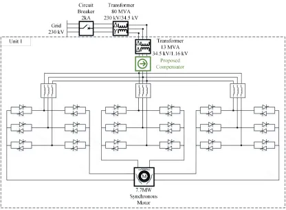
4.1 System Under Study . . . 42
4.2 Simulation Result . . . 42
4.3 Power Quality Criteria . . . 48
4.4 Real-time (RT) Implementation of the Tri-window Compensator . . . 49
4.5 Summary . . . 52
Chapter 5 Practical Considerations . . . 58
5.1 Design and Cost Analysis of the Reactive Compensator (SVC) . . . . 58
Chapter 6 Toward Distributed Compensation: Power Qual-ity Improvement inside Microgrids. . . 64
6.1 Harmonic Node-Analysis of Microgrids . . . 65
6.2 Fundamental of Voltage Compensation . . . 69
6.3 System Under Study . . . 76
6.4 Results and Discussion . . . 77
Chapter 7 Conclusion . . . 80
Bibliography . . . 82
Appendix A T F DI Convergence to the T HD for Periodic Loads 89
Appendix B Proof of Equation (3.18) . . . 92
Appendix C C-code Demonstration. . . 95
List of Tables
Table 4.1 Load description and power quality indices before and after the
compensation. . . 47
List of Figures
Figure 1.1 Typical structure of a passive filter. . . 6
Figure 1.2 Popular structures of SVCs. . . 9
Figure 1.3 Typical structure of an active filter. . . 10
Figure 2.1 Frequency domain difference between the non-periodic and pe-riodic quantities. . . 25
Figure 2.2 Demonstration of an amplitude-modulated waveform. . . 28
Figure 3.1 The tri-window structure of the proposed method. . . 31
Figure 3.2 Structure of the proposed compensator. . . 32
Figure 3.3 Flowchart of the adaptive fuzzy algorithm for modification of slow compensator window length. . . 40
Figure 3.4 Frequency response of the moving average integrator for differ-ent window lengths. . . 41
Figure 3.5 The bandwidth of the current waveform after the fast compen-sation with different window lengths. . . 41
Figure 4.1 The circuit diagram of the steel mill cycloconverter. . . 43
Figure 4.2 Current waveform for four loading cases of the cyclo-converter and their corresponding current after the compensation . . . 44
Figure 4.3 Result of the slow compensator for loading case 1. . . 55
Figure 4.4 Real-time test setup schematic. . . 56
Figure 4.4 Test results. . . 57
Figure 5.1 Desired real-time platform for development of the tri-window
compensator. . . 59
Figure 5.2 Static VAR Compensator designs used for performing cost analysis. 60
Figure 6.1 Typical microgrid structure with fuel cell, photovoltaic, and wind turbine generation, and electric vehicle and other
non-linear loads. . . 66
Figure 6.2 The node-analysis representation of the grid connected microgrid 67
Figure 6.3 Structure of the proposed shunt harmonic and unbalance
com-pensation technique. . . 74
Figure 6.4 The frequency response of the proposed RDFT filter. . . 75
Figure 6.5 The filter for the extraction of the voltage harmonic. . . 76
Figure 6.6 Schematic of the system under study used to test the proposed
technique . . . 76
Figure 6.7 The time-line of different events in the simulation. . . 76
Figure 6.8 Power quality criteria, without compensation, with compensa-tion by distributed control, and with compensacompensa-tion by
central-ized control . . . 78
Figure 6.9 The RMS current of the active filter units with and without the
centralized controller. . . 79
Figure D.1 (a) Real-world current waveform (loading case 4), (b) current
Chapter 1
Introduction
Current distortion has a harmful effect on both distribution system equipment
and on loads that the system supplies. Because of this, current distortion is a main
cause of supply quality degradation. Furthermore, current distortion increases the
root mean square value of current without increasing energy transmission. Thus,
it creates increased losses during transmission of energy as well as requiring higher
ratings of distribution system equipment. Therefore, it is necessary to reduce
cur-rent distortion for the same reasons as for reactive curcur-rent, as well as to reduce the
other harmful effects. If distortion exceeds some limits, then equipment is needed
for its suppression. “Compensator” is a term used for the equipment that mitigates
the effect of power quality degrading loads. There are numerous types of devices
and strategies available for the compensation of distorted but periodic currents from
harmonic generating loads. However, although non-periodic loads, result in similar
harmful effects, there has been very limited research on how to compensate them.
The focus of this research is to combine the recent advances in power electronics and
signal processing to manage and compensate non-periodic loads.
In this chapter, different some key concepts related to compensation are discussed.
These concepts are (1) power quality, its issues, and indices, (2) power quality
im-proving devices (compensators), (3) power theories, (4) time-frequency distribution,
1.1
Power Quality (PQ)
In general, a power system quality disturbance is defined as “ Any power
prob-lem manifested in voltage, current, or frequency deviations that results in failure or
misoperation of customer equipment” [1]. We can add to this definition the problems
that result in a decrease in the efficiency of the power systems. PQ is, therefore,
defined as the absence or limited presence of power quality disturbances. Keeping
the quality of power within the acceptable range has been one of the most
challeng-ing tasks of the utilities and device manufacturers. Especially, by the recent large
increase in non-linear loads (power electronics based) and grid-connected distributed
generation the PQ issues been worsened. It is shown that the keyword “Distributed
Generation” is the fifth most used phrase in articles regarding the power quality [2].
The power quality could be seen from two aspects, the from the utility side, and
from the costumer side. First, the utility is responsible for providing a supply voltage
which is balanced, constant, sinusoidal, and with a fixed frequency (60 Hz in the
United States). However, a little deviation from this condition is also acceptable
by the standards. Improving this “voltage quality (VQ)” is the responsibility of the
utility companies, and remarkable deviation from this power quality would result in
failure and mal-operation of power systems and the loads. Some examples of such
power quality disturbance are voltage sag [3], voltage swell [4], voltage interruption[5],
voltage harmonic [6], voltage imbalance [7], voltage flicker [8], voltage transient [9],
and frequency deviation[10].
The second perspective of the power quality is the consumer side. The customer is
responsible for drawing a current waveform which has the same shape as the voltage
waveform with possibly different magnitude. In other words, for a system with a
si-nusoidal voltage supply, the current waveform of the load should have the same phase
conduc-tance and zero equivalent suscepconduc-tance). Any load that does not have balanced pure
resistive characteristics is considered a PQ degrading load. Though small deviation
from this condition is acceptable, larger variation results in a decrease of the power
system efficiency. This lower efficiency is the product of several factors; increase in
the power loss, elevation of the source current RMS, and elevation of the line voltage
distortion. As a result, the customers with unacceptable “current quality (CQ)” will
end up paying penalties to the utility. Some example of the CQ disturbance are load
reactive power [11], load harmonic [12], unbalance load [13], load inter-harmonic [14].
It is noted that CQ disturbances could lead to VQ disturbances and vice versa.
For example, large load current drawn from a non-linear load would result in a
signif-icant voltage drop on the line impedance, which in turn results in distorted voltage
waveform. On the other hand, also, the distorted voltage on a balanced resistive load
would also lead to current waveform distortion. Therefore, it is the responsibility of
the utility to provide voltage supply with acceptable VQ and then the responsibility
of the consumers to maintain acceptable CQ. It is noted that the primary purpose of
this dissertation is the improvement of the CQ disturbances which are the
byprod-uct of large steel mills. However, in the last part of the dissertation, a possible VQ
disturbance improvement for the microgrids (MG) is also proposed.
1.1.1
Power Quality Indices
In general, the indices used to evaluate the quality of power are categorized into
three groups, namely, waveform distortion indices, equivalent susceptance indices,
and sequence indices.
The first group of PQ indices is waveform distortion indices that are used for both
VQ and CQ disturbance evaluation. The most famous index in this group is the “Total
Harmonic Distortion (THD)” index which is used to quantify the level of harmonic
of the fundamental frequency). THD is calculated using the following equation:
T HD = v u u t
P∞
n=0 X(nω0)2−X(ω0)2
X(ω0)2
% (1.1)
where X is the quantity of interest (current or voltage), ω0 is the fundamental
fre-quency inrad/s, andnis the harmonic order. Other indices in this category are crest
factor [15], notch area (and notch depth) [16], and instantaneous distortion energy
ratio [17].
The second group of power quality criteria is the equivalent susceptance indices.
For a load to receive the required active power with the highest efficiency, it is
nec-essary that its equivalent susceptance is equal to zero. It is noted that the
equiv-alent susceptance (Be) is proportionally related to the reactive power consumption
(QL=Be×V2). The most popular power quality index in this category is the power
factor (P F) which is calculated as follows:
P F = P
S =cos(ϕ) (1.2)
where P is the load active power, S is the load apparent power, and φ is the phase
displacement between voltage and the current waveform. It is noted that this
def-inition holds meaning only for sinusoidal and balanced systems [18]. Other indices
in this group are displacement factor, interactive power transfer factor, and reactive
power transfer factor [19]. It is noted that this group of power quality indices is
mainly related to CQ disturbances.
The third group of power quality criteria, sequence indices, are evaluating the
level of balance in the power system and loads. Therefore, these indices are also
working for both CQ and VQ disturbances. They are called sequence indices since
any imbalance in power system could be reflected in the existence of negative and
zero sequence components of voltage or current [20]. The most popular power quality
U FX =
XN
XP (1.3)
where X is the quantity of interest, N superscript demonstrates the negative
se-quence, andP superscript demonstrates the positive sequence. some other indices in
this group are V U N B and IU N B proposed in [21].
Although the existing PQ indices are capable of describing the level of PQ
distur-bance in most of the normal loads and network, for some especial cases, such as for
the loads from steel mills, these PQ indices lose their meaning. Chapter 2 is dedicated
to the discussion on the difference between non-periodic loads (such as steel mills)
and periodic loads. Moreover, a new set of PQ indices is proposed that are capable
of evaluating this situation.
1.2
Power Quality Improving Devices
Various technologies have been developed to address the PQ disturbances and
bring the power system state back within the acceptable PQ indices. These devices
are divided into two basic categories, passive devices, and active devices. Passive
devices are always pre-designed based on the power system condition to mitigate
some PQ disturbances partially. Active devices, on the other hand, adaptively modify
their behavior to comply with the changes in the system configuration, loading, or
generation. The power quality improving devices are called compensators. In this
section passive and active compensators are introduced in more details.
1.2.1
Passive Compensators
Passive compensators could be divided into four categories: (1) power factor
cor-rection devices, (2) harmonic reduction devices, (3) voltage profile improvement [22].
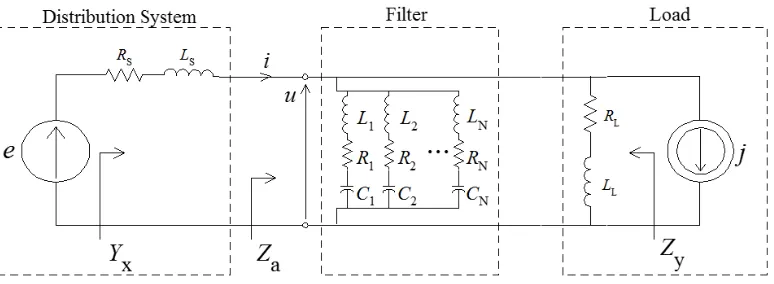
Figure 1.1: Typical structure of a passive filter.
shunt capacitors and shunt inductors used to improve the CQ of the load. They are
designed to generate (or consume) the reactive power that the load consumes (or
generates). The rating and values of these components are pre-calculated, and they
are installed, usually, at the load terminal. The problem with these compensators is
their unresponsiveness to the load changes and system changes [23]. Moreover, they
might result in resonance with the line impedance.
The second group of passive compensators, harmonic reduction devices (also
known as passive filters), are mainly shunt tuned LC filters that are designed to make
an extremely large conductance path for current harmonics. Fig. 1.1 demonstrates
the equivalent circuit for one phase of a passive filter connected to a harmonic
gen-erating load in the distribution system. These filters require one series RLC branch
for each harmonic are eliminating. Though these devices are cheap and reliable for
most periodic loads, they tend to become ineffective for loads with more complicated
harmonic patterns (such as non-periodic loads).
The third group of passive compensator is voltage profile improvement devices.
These devices are (switched) capacitor- and inductor banks located in both
distri-bution and transmission network to compensate for loads with large reactive power
transactions and Ferranti effect [24]. Both of these situations result in exceeding the
voltage magnitude beyond acceptable voltage level. These compensators can be shunt
1.2.2
Active Compensators
Active compensators are capable of adaptively track the PQ disturbances.
There-fore, they are responsive to the change in loads and network configuration. These
compensators are divided into three groups: Static VAR Compensators (SVCs), Static
Series Compensators, and Switching Compensators.
The first class of active compensators, SVCs are adaptive susceptances. They
use a combination of passive elements (inductors, capacitors, and resistors) and
ac-tive devices (Thyristors) to form a controlled susceptance. SVCs are mainly used to
compensate for reactive power generation/consumption. Moreover, more heuristics
structures of SVCs can also compensate unbalanced power. The main drawback of
the SVCs is the fact that the use of switching components results in the generation of
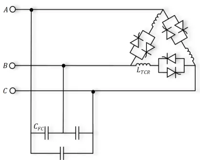
harmonic current, which in some cases are fairly large. Fig. 1.2 demonstrates three
popular structures of the SVC. In this dissertation, we perform a cost analysis to
explore the most optimal structure for the development of our technique.
The first structure of SVC, FC-TCR (fixed capacitor- thyristor controlled reactor),
shown in Fig. 1.2a is capable of compensating reactive power [25]. However, it
gen-erates current harmonics of the order 6k±1 multiples of the fundamental frequency.
Moreover, this compensator is incapable of compensating the unbalanced power. The
second structure, 12-pulse FC-TCR is shown in Fig. 1.2b. This device consists of
one Y −Y and one Y −∆ transformer that together reduces the harmonic content
of the reactive compensator to 12k±1 multiples of the fundamental frequency [25].
However, similar to the basic FC-TCR, 12-pulse FC-TCR is incapable of
compensat-ing the unbalanced power. The third structure, adaptive balanccompensat-ing compensator, is
shown in Fig. 1.2c. This configuration is an extension of the FC-TCR that is also
capable of compensating the unbalanced part of the current [26]. However, since for
should be different, the triple-nth harmonics generated by the TCR branch could
not circulate inside the delta connected compensator and will be injected into the
line. Therefore, although this compensator is capable of compensating the
unbal-anced power, it generates and injects 2k±1 multiples of the fundamental frequency
to the grid.
The second class of active compensators is Static Series Compensators. These
compensators are mainly used to mitigate the subsynchronous resonance [27, 28],
controlling the transmitted power [29], and preventing loop flows.
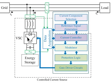
The last class of active compensators, switching compensators (also known as
active filters) are controlled current sources. The basic structure of an active filter
is shown in Fig. 1.3. When a voltage source converter is accompanied by a proper
control algorithm, it could behave as a controlled current source. Therefore, assuming
enough bandwidth and rating, it would be able to compensate harmonics, reactive
current, and unbalance current. Therefore, if this current source is controlled to
generate the distortion part of the current in the opposite direction, active filter
compensates the load.
The most important subsystem within the control structure of an active filter is the
“reference signal generation” block which is responsible for calculating the distortion
part of the current. Various “Power Theories” have been developed to calculate this
distortion part of the current, which will be discussed briefly in Section 1.3 below. It
is noted that the main focus of this dissertation is to develop an appropriate reference
signal generation block, that is capable of compensating different part of the current
waveform of the non-periodic loads.
1.3
Power Theories
Power theories are mathematical techniques used for decomposing the current
avail-(a) Fixed capacitor thyristor controlled reactor (FC-TCR)
(b) Fixed capacitor 12-pulse thyristor controlled re-actor.
(c) Adaptive balancing compensator.
Figure 1.3: Typical structure of an active filter.
able technologies. These current (power) components could be utilized for different
applications, such as energy metering, compensation, performance evaluation, and
system design [18]. Moreover, depending on the design requirement, and available
technologies, different power theories might be suitable for various applications. In
this section, the main power theories developed for the application purposes are
dis-cussed.
References [30] and [31] provide comprehensive reviews on the power theories
uti-lized by different active filters. Morsi et al. [18], also, investigate the power theories
using bottom-up and top-down approaches. These power theories are placed into
three subcategories, namely, time-domain based methods, frequency domain based
1.3.1
Time-domain power theories
The time-domain based power theories decompose the current waveform into its
orthogonal components without using mapping the power components (voltage and
current) to any other domains (e.g. frequency, time-frequency, wavelet). Most
well-known time domain power theories are Fryze power theory and instantaneous pq
power theory.
Fryze theory takes advantage of the fact that the only part of the current
wave-form which is contributing to the power transfer has the same shape as the voltage
waveform [32]. Therefore, this theory simply divides the load current into two parts,
the active current, which is responsible for the power transfer, and the non-active
part which does not contribute to the transfer:
p(t) =v(t)iL(t)⇒instantanous power (1.4)
P = 1
T
Z T
0
p(t)dt ⇒active power (1.5)
Ge=
P VRM S2
⇒equivalent conductance (1.6)
ia(t) = Gev(t)⇒active current (1.7)
The remaining part of the current is named non-active current (ina(t) = iL(t)−
ia(t)). This part does not contribute to the power transfer and needs to be
compen-sated using the active filter. It is noted that the advantage of the Fryze theory is its
simplicity. However, using Fryze theory, the optimum utilization of bandwidth and
rating of the active filter and also the integration of active filter with other devices
are not possible.
The second popular time-domain power theory is the instantaneous pq power
theory [33]. This theory has been widely used for the control of power converter
due to its simplified design and high-speed [34].This power theory first transfers the
transform.
vαβ0 =T vabc (1.8)
iαβ0 =T iabc (1.9)
where v and i are voltage and current vector, respectively. abc and αβ0 subscript
demonstrate the vector in the abc and rotating domain, respectively. T is the Park
domain mapping matrix calculated as follows:
T = s 2 3
cos(θ) cos(θ− 2π
3 ) cos(θ+ 2π
3 )
sin(θ) sin(θ− 2π
3 ) sin(θ+ 2π 3 ) √ 2 2 √ 2 2 √ 2 2 (1.10)
where θ is the rotation angle of the rotating frame.
After mapping the quantities into the rotating frame, the instantaneous powers
are calculated as follows:
p0 p q =M i0 iα iβ (1.11) M = s 2 3
v0 0 0
0 vα vβ
0 vβ −vα
(1.12)
where pis known as instantaneous real power and consists of constant (¯p) and
oscu-lating (˜p) parts; q is known as instantaneous imaginary power which also consists of
constant and oscillatory parts (q = ¯q+ ˜q); and finally, p0 is known as the
instanta-neous zero-sequence power (p0 = ¯p0+ ˜p0).
It is shown that among these six power components (¯p, q,¯ p¯0, and ˜p, q,˜ p˜0), only
constant part of the real power contributes to the power transfer (¯p). Therefore,
to the five power components that are not contributing to the power transfer. The
voltage source converter generates this value to annihilate the distortion part of the
current. The reference current is calculated as follows:
iαβ0∗ =
i0 iα iβ
=M−1
˜ p0 ˜ p q (1.13)
ic∗ =T−1iαβ0∗ (1.14)
Though the instantaneous pq power theory is simple and fast, it loses its reliability
for compensating the various abnormal loadings, such as non-periodic loads.
1.3.2
Frequency-domain power theories
The second class of power theories are frequency-domain based. They require the
preprocessing of the data and mapping from the time domain to the frequency domain.
Th most popular power theory in this class is the Current Physical Component theory.
In this technique, the non-active part of the current is further decomposed into four
parts, reactive, unbalanced, scattered, and generated [35]. It is suggested that each
part of the non-active current can be compensated separately. The technique is
similar to the Fryze theory up to the point that it calculates the active current. The
remaining current are calculated as follows:
ir =
√
2Re{X
n∈N
jBenUnejnω1t} ⇒reactive current (1.15)
iu =
√
2Re{X
n∈N
AU#ejnω1t} ⇒unbalanced current (1.16)
is =
√
2Re{X
n∈N
(Ge−Gn)Unejnω1t} ⇒scattered current (1.17)
ig =
X
h∈(Ni∩N¯v)
where Ge is the load equivalent conductance, U is the voltage phasor, U# is the
voltage phasor transpose, Ben is the equivalent susceptance of each harmonic, A is
the unbalanced admittance,Gn is the harmonic equivalent conductance. N is the set
of harmonic orders in voltage and current,Ni is the set of harmonic orders in current,
and Nv is the set of harmonic orders in voltage.
The decomposition of the current waveform into several components is very helpful
for sharing the rating and bandwidth between different compensators. However, for
some abnormal loading cases, such as non-periodic loads, the definition of frequency
components using solely FFT is not efficient anymore. The reason is that these
loads do not only contain multiple integers of the fundamental frequency components.
Therefore, the CPC theory would become ineffective in such cases. Moreover, in the
case that the voltage waveform is more distorted than the current waveform, the CPC
theory would increase the line current distortion.
1.3.3
Hybrid-domain power theories
Hybrid time-frequency algorithms combine time and frequency domain approaches.
Czarnecki et. al [36] proposed a hybrid active filter that consists of a frequency
do-main method for the compensation of reactive powers and a time-dodo-main method for
the compensation of non-periodicity. Such techniques are, however, more complex,
not verified for non-periodic current compensation, and may increase the line current
THD in the case of a highly distorted supply voltage.
1.4
Time-Frequency Analysis (TFA)
TFA was motivated by the need to describe non-stationary signals, where Fourier
transform proves ineffective. Non-stationary signals are the ones whose frequency
representation methods are designed to mathematically describe these signals, namely
short time Fourier transform (STFT), Wigner-Ville distribution (WVD), and
Choi-Williams distribution (CWD) [37]-[38]. To systematically design proper time-frequency
distribution (TFD), Cohen generalization of the quadratic TFDs is used [37]. Cohen
proved that one can relate the desirable properties of TFDs to constraints on its
kernel:
T F Ds(t, ω) =
1 4π2
Z Z Z ∞
−∞IACs
(u, τ)φ(θ, τ)
×e−jθt−jτ ω+jτ udθdτ du (1.19)
where φ(θ, τ) is a two dimensional function (in Doppler-lag domain), called kernel
and T F Ds is the time-frequency distribution of the signal. The constant time cross
section of time frequency distribution (T F D(t0, ω)) represents the frequencies
avail-able at time t0, and its frequency cross section (T F D(t, ω0)) represents the times
when frequency ω0 occurred. And IACs is theinstantaneous auto-correlation of the
signal s(t), respectively. IACs is defined in Eq.(2.2).
IACs(t, τ) = s∗(t−τ /2)s(t+τ /2) (1.20)
The desirable properties of TFD and their constraints are defined as follows:
Time Marginal
Integration of the TFD over frequency gives the “Instantaneous Power” (|s(t)|2):
Z ∞
−∞T F Ds(t, ω)dω =|s(t)|
2
⇐⇒φ(θ,0) = 1 (1.21)
Frequency Marginal
Integration of the TFD over time gives the “Energy Spectrum” (|S(ω)|2):
Z ∞
−∞T F Ds(t, ω)dt=|S(ω)|
2
Global Energy
Integration of the TFD over the entire time-frequency plane yields the “Signal
Energy” (ES):
Z ∞
−∞ Z ∞
−∞T F Ds(t, ω)dtdω=Es⇐⇒φ(0,0) = 1 (1.23)
Reduced Interference
Due to the bi-linearity of the IAC, introducing “artifacts” (interference) is
in-evitable in generating TFDs. If the kernel has low pass filter characteristic in
Doppler-lag domain (θ, τ), the interference could be reduced.
Since the disturbances in power systems are characterized by the presence of multiple
frequency components over a short duration of time, keeping high time-frequency
resolution, while avoiding artifacts is of great significance in their analysis [39].
Although WVD satisfies the first three constraints (φ(θ, τ) = 1), a large proportion
of interference could result in a poor interpretation of a signal. However, in the case
of analyzing non-periodic current, since it is the energy of harmonics in different
time-windows and frequency windows that are important, the reduced interference
requirement could be waived. Therefore, for the analysis of the non-periodic load
current, the WVD is chosen.
1.5
Non-periodic Load
In general, any power system quantity (voltage, current) whose frequency content
is not integer multiples of the system supply frequency (i.e. 50 Hz, 60 Hz) is
con-sidered a non-periodic quantity [40]. The time duration of the non-periodicity could
be from a fraction of one period of the power system frequency up to a steady state
Non-periodicity in a power system shall not be confused with the mathematical
meaning of periodicity. In the mathematical sense, a signal is considered
non-periodic if it does not have a complete pattern within a measurable constant time
frame. To reconcile the definition of the non-periodic signal in power systems and
mathematics, Czarnecki [36] proposed a classification of the waveforms based on their
periodicity, as it relates to the power system generators, namely, co-periodics,
non-coperiodics, and quasi-periodics. A co-periodic quantity has an integer multiple of
the power system frequency. On the contrary, a non-coperiodic quantity is a periodic
or non-periodic waveform that does not have the same period of the power system
generators or any of its multiples. If the non-coperiodic current has a small time
du-ration and small magnitude comparing to the fundamental component of the signal, it
is called quasi-periodic. The frequency spectrum of a quasi-periodic current, though
continuous, is located in the sub-band neighborhood of the fundamental frequency
(and its multiples) [41]. In this work when the term “non-periodic” is used, it means
non-coperidoic.
Non-periodic current could be the result of various loads, such as cyclo-converters,
welders, arc furnaces, adjustable speed drives [42]. The harmful impacts of the
non-periodic currents are similar to those of harmonic loads, such as contribution to power
loss, elevation of the source current RMS, interference with the local sensitive loads,
elevation of the line voltage distortion, and interference with measurement devices
[43].
Two widely used devices for load current compensation are active filters and
pas-sive filters [36]. Paspas-sive filters, though straightforward and inexpenpas-sive as compared
to active filters, may bring a strong possibility of the amplification of inter-harmonics
noise components of the current, which makes them not practically applicable for
non-periodic load compensation. Therefore, active filters (switching compensators)
Time-domain based approaches are mostly originated from the Fryze power theory
[32]- [44], instantaneous p-q theory [45, 46, 34] , and synchronous d-q frame theory
[47]. In [48] and [49] an extension of Fryze power theory, and instantaneous power
theory is utilized for the compensation of non-periodic current. The time-domain
based techniques have the advantage of being simple and instantaneous under some
specific conditions.
The second group of power theories, frequency domain approaches, are based on
the Fourier transform or Kalman filtering of the current or voltage waveforms. In [50],
Czarnecki proposed a frequency based method to decompose the load current into
ac-tive, reacac-tive, scattered, and generated current. Unlike the time-domain approaches,
frequency based methods are more easily tailored to compensation objectives.
How-ever, they are not instantaneous, and they are more complex due to the necessity of
FFT calculation of each harmonic.
1.5.1
Existing Techniques for Non-periodic Current Compensation
Compensation using Fryze theory
One of the earliest power theory to describe the power flow and decomposing the
current waveform into orthogonal components is proposed by Fryze in [32]. In fact,
the first time the term “power theory” is utilized was in that article. Fryze power
theory decomposes the current waveform into active and non-active components;
where the active component is the part of the current which is responsible for power
transmission, and the non-active component is any part of the current that does
not contribute to the power transfer and need to be compensated. Fryze theory has
been used for different applications such as reactive current compensation, harmonic
In [48], Fryze theory is proposed for the compensation of non-periodic load current.
This technique considers all the non-periodicity, harmonics, reactive current, and
imbalance current as a residual non-active current. However, the feasibility of a
device that is capable of such compensation is not discussed. Moreover, the proposed
technique utilizes an arbitrary averaging window length for the calculation of reference
current. The dissertation suggests a trade-off between averaging window length and
the cost of the compensator.
Compensation using pq theory
The instantaneous pq theory, also known as instantaneous active and reactive
power theory, is first proposed by Akagi in 1983 [33]. The pq theory performs a
Clark transformation of current and voltage waveforms to define “instantaneous”
active (p) and reactive (q) powers, and subsequently reactive and active current. pq
theory has been widely used in the compensation of power quality degrading events,
such as non-linear loads, imbalance loads, and systems with non-sinusoidal voltage
supply [34, 51].
In [45], the pq theory is proposed for the compensation of non-periodic loads.
In this technique, an integrator with “averaging time tending to infinity” is used.
Moreover, it is mentioned that a faster compensation of non-periodic current comes
at the price of “power fluctuation”, and “ torque ripple in the axis of the generator”.
As a result of this trade-off between fluctuation and speed, the technique required
a decision making to be performed by engineers before setting up the compensator,
which largely decreases its objectivity. Therefore, it is evident that the pq-theory
based compensation is incapable of efficiently addressing the non-periodic load current
Compensation using Current’s Physical Components theory
Another power theory utilized for the compensation of power quality degrading
loads is proposed by Czarnecki, known as Current Physical Components (CPC) theory
[50]. In this technique, the current waveform is decomposed into several components,
each carrying a physical meaning, namely, active current, reactive current, scattered
current, generated current, and unbalance current. CPC theory has been used for
the compensation of various power quality degrading situations, namely, non-linear
load, unbalanced load, pulsed loads, and systems with non-sinusoidal and imbalance
supply voltage[52].
In [41], the CPC theory is used for the compensation of loads with the non-periodic
voltage of a finite energy. For the CPC theory to be able to decompose such a load
into the orthogonal components (active current, reactive current, and scatter
cur-rent), several optimistic assumptions are made, such as infinite window length of the
calculation, and continuity and finite energy of the voltage signal. Also, the proposed
technique minimizes the source current only by minimization of the reactive current
and not considering other components of the current.
In another work, CPC theory is utilized to compensate the non-periodic current
using a hybrid time and frequency domain based compensator[36]. In this work
the current components are compensated using two compensators; one (a thyristor
controlled susceptance) responsible for reactive current and imbalance current
com-pensation, and another (active filter) responsible for harmonic current and the rest
of the non-periodic current. Lumping all the harmonic and non-periodic part of
the current into “residual component”, however, degrades the meaning of Current
Physical Components. In other words, the non-periodic part of the current does not
carry a physical meaning and is not compensated by a compensator that is designed
specifically for such current waveform. Moreover, the proposed technique is incapable
cur-rent waveform. Also, this method is not evaluated using the existing power quality
criteria, as they are incapable of describing the non-periodic load.
Shortcomings of the Existing Techniques
The existing techniques for the compensation of the non-periodic load demonstrate
several shortcomings listed below:
1. Single calculation window:
Non-periodic load current consists of numerous quasi-harmonic components, and
inter-harmonic noise. Therefore, unlike the frequency components of a periodic
quantity, it might not share a greatest common divisor frequency. Moreover, there
exists a large difference between the frequency of load various components of
cur-rent to be compensated. Therefore, choosing a single value for the calculation
window, which takes into account such variety of frequency components, largely
decreases the efficiency of the existing techniques. In other words, in order to
compensate the non-periodic current solely, based on the existing power theories,
requires a voltage source converter with an extremely large rating, and
simultane-ously extremely large bandwidth. Therefore, an efficient technique would be able
to decompose the current waveform into different frequency bands with different
time window lengths.
2. Energy storage requirement:
Compensation of non-periodic current requires active current injection. The reason
is that the frequency components of the non-periodic load are not all multiple
integers of the fundamental frequency. Therefore, there will be excess or deficient of
active power over one cycle of power frequency which should be provided using an
energy storage. The existing technique, however, does not consider such constraint
size which is one of the most salient cost factors of the design of non-periodic load
compensator.
3. Decomposed components without meaning:
All of the existing techniques are the mere extension of the techniques
assum-ing periodic quantities. Therefore, the decomposed current components lose their
meaning migrating from periodic quantities to non-periodic ones. An efficient
technique for the compensation of non-periodic current would take into account
the differences between periodic and non-periodic quantities while using the same
framework used for the compensation of periodic quantities. Therefore, such
tech-nique has to decompose the current into components that are meaningful parts of
the non-periodic current. As a result, it is possible to develop devices which are
specifically designed to compensate each part of such current.
4. Absence of power quality indexes:
None of the proposed techniques are evaluated using power quality indexes. The
main reason is that most of the power quality indexes are explicitly defined based
on the assumption of the periodicity of power quantities. An acceptable power
quality index takes into account the difference between non-periodic and periodic
quantity but is capable of describing the characteristics of both systems.
1.6
Contribution of this Dissertation
The method proposed in this dissertation is a hybrid time-frequency method
to provide current reference for a co-located arrangement which is temporally
dis-tributed. This compensation technique consists of three parts, namely fast
compen-sator, slow compencompen-sator, and reactive compensator. The first (fast compensator) and
second (slow compensator) are time-domain based approaches and the third (reactive
component compensator) is a frequency based method. The proposed technique is
sup-ply, capable of compensating the unbalanced loads and poly-phase loads. Moreover,
the design limitation of the proposed method, such as the active filter energy
stor-age requirement, is discussed thoroughly. The proposed technique is validated using
MATLAB simulation in conjunction with real-world data acquired from a steel mill
cyclo-converter. Moreover, a real-time controller in the loop structure is utilized to
verify the method using steel mill data. It should be noted that compared to the
existing techniques of compensation of non-periodic loads, the proposed technique
utilized faster and more sophisticated signal processing tools.
Moreover, three power quality indexes are proposed to develop supervisory
con-trol for the compensators and also evaluate the proposed technique. Three signal
processing driven criteria, namely, modulation index, time-frequency distortion, and
high frequency distortion index, are proposed to comply with the non-stationary
be-havior of the non-periodic load. Existing power quality criteria, such as Power Factor
(PF) and Total Harmonic Distortion (THD) are incapable of describing the
charac-teristics of non-periodic loads. The proposed approach demonstrates high capability
in improving these power quality indexes.
This dissertation is organized as follows: Chapter 2 and Chapter 3 describe the
development toward the proposed technique, Chapter 4 demonstrates the simulation
and real-time results of this technique, Chapter 5 describes the practical
considera-tions of building this technique, and Chapter 6 discusses the possible future works
based on the development presented. Moreover, this dissertation is followed by four
Chapter 2
Non-periodic Current Properties and Power
Quality Indexes
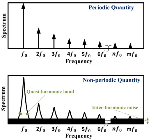
A general frequency spectrum of a periodic and a non-periodic load are depicted
in fig. 2.1. Loads with non-periodic current share two characteristics representable
in the frequency domain [36]. First, instead of sharp spikes around the harmonic
frequencies, the non-periodic current has rather a narrow band of frequencies around
each harmonic, which is referred to as a “quasi-harmonic band”. This part of the
current results in a variation of the current waveform peak based on an envelope.
This phenomenon could be modeled as an amplitude modulation of the component
by a time-varying carrier. Any device for the compensation of this part of the
cur-rent waveform requires a large window length (integer multiple of the fundamental
frequency cycle) to be able to catch and filter the low frequency components of the
signal. In the next chapter a high rating low bandwidth compensator is proposed for
the compensation of such quasi-harmonic band of the spectrum.
The second frequency domain feature of non-periodic components is the
pres-ence of non-negligible frequency content between different harmonics, which is called
“inter-harmonics noise” [36, 53]. These components could be amplified drastically if
a traditional resonance based passive filter is used to compensate them. Therefore,
extraction of a compensator control reference targeted toward this feature of the
non-periodic components should have small window length (fraction of the fundamental
Figure 2.1: Frequency domain difference between the non-periodic and periodic quan-tities.
waveform. In the next chapter, a compensator named fast compensator is proposed
for such purpose.
There is also a need for the elimination of reactive part of the current waveform,
which is common between most of the power quality degrading loads. The window
length required for the calculation of the reactive part of the current is equal to the
fundamental frequency cycle.
As demonstrated in fig. 2.1, since the spectrum of the non-periodic current
con-tains frequencies other than the power system frequency (e.g. 60 Hz) and their
multiples, the well-known total harmonic distortion would result in an inaccurate
representation of the harmonic distortion level. Moreover, the non-periodic current
is non-stationary, which means its frequency spectrum demonstrates temporal
varia-tion. Therefore, it cannot be quantified using frequency-domain based power quality
indexes. To alleviate these issues, three power quality indexes, capable of describing
2.1
Time-Frequency Distortion Index (
T F DI
)
In this work, a time-frequency based index is proposed to demonstrate the level
of current distortion. Time-frequency domain analysis takes into account the time
and frequency domain simultaneously [54]. Time-frequency based criteria has been
recently utilized to define the active/ reactive part of the power (current) waveform
[55]. In this work, the time-frequency analysis is used to describe the non-fundamental
part of the current waveform. Similar to T HD, T F DI emphasizes the total power
of the waveform excluding the power in the fundamental frequency of the current. In
this work, Wigner-Ville time-frequency distribution (WVD) of the current waveform
is used for the definition of the T F DI. The WVD distribution, W V Ds(t, ω), of the
current waveform,s(t), is calculated using the following equation:
W V Ds(t, ω) =
1 4π2
ZZ Z ∞
−∞
IACs(u, τ)φ(θ, τ)
×e−jθt−jτ ω+jτ udθdτ du (2.1)
where φ(θ, τ) is a two dimensional function,φ(θ, τ), (in Doppler-lag domain), called
kernel. It is equal to “1” for the WVD. t and ω are time and frequency, respectively,
and IACs is the instantaneous auto-correlation of the signal s(t) defined as:
IACs(t, τ) = s∗(t−τ /2)s(t+τ /2) (2.2)
The WVD could be used to extract the frequency and time localization of the
current waveform, which are necessary to define a criterion for non-periodic currents.
This capability comes from the fact that WVD meets two requirements, namely, time
marginal (TM), and frequency marginal (FM). These requirements are described as
T M : Z ∞
−∞
W V Ds(t, ω)dω=|s(t)|2 (2.3)
F M : Z ∞
−∞
W V Ds(t, ω)dt=|S(ω)|2 (2.4)
The signal energy (ES) over the window of calculation (T) is calculated using the
following equation:
Es =
1
T
Z ωmax
0
Z T
0
W V Di(t, ω)dtdω (2.5)
where ωmax is the largest frequency components of the signal which is based on the
Nyquist–Shannon theorem equal to half of the sampling frequency.
The energy of the fundamental harmonic, Es1, (which is responsible for the actual
transfer of power from the source to the load) is calculated using the following
equa-tion.
Es1 =
1
T
Z ω0+ε
ω0−ε Z T
0
W V Di(t, ω)dtdω (2.6)
where ε is considered a few frequency bins in the neighborhood of the fundamental
frequency.
Finally, the time-frequency distortion index is defined as:
T F DIs=
s
Es−Es1
Es1
% (2.7)
Note that, for periodic quantities, this definition coincides with the traditional
definition of total harmonic distortion calculated using Fourier transform (Eq. 2.8).
On the other hand, THD loses its efficiency for calculating the harmonics distortion
of the non-periodic (non-stationary) signal.
T HDs =
v u u t
P∞
n=0 I(nω0) 2
−I(ω0) 2
I(ω0)
Figure 2.2: Demonstration of an amplitude-modulated waveform.
Please refer to Appendix A for the discussion about the equality of T HD and
T F DI for periodic components.
2.2
Modulation Index (
m
i)
As demonstrated in [36], one of two main characteristics of non-period currents,
besides the existence of inter-harmonic noise, is the presence of some form of
am-plitude modulation which results in spreading the frequency content around each
harmonic. In this work, modulation index, defined in (2.9), is utilized as a fast
time-domain method to demonstrate the level of amplitude modulation, and therefore the
degree of the non-periodicity of the current. Assume that the current waveform of a
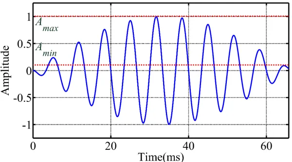
non-periodic current is depicted fig. 2.2. The modulation index, mi, for such a case
is calculated as:
mi(t) =
Amax−Amin
Amax+Amin
(2.9)
where Amax and Amin are the maximum value of the modulated signal envelope,
respectively.
One of the main advantages of modulation index criterion, compared to the
the modulation frequency. On the other hand, to calculate the frequency based
crite-ria, such as distortion factor [40], at least on the period of the modulation frequency
is needed.
2.3
High Frequency Distortion Index (
HF DI
)
The existing criteria, T F DI and mi are appropriate to access the overall
perfor-mance of a compensator for non-periodic currents. For the purposes of evaluating the
performance of compensation within a particular frequency range another metric is
developed. This is important since compensation may be done is frequency intervals
depending on the power ratings and bandwidth limitations of particular equipment.
Thus, a targeted index, typically in the high frequency where compensation is more
limited is useful. For such purpose, High Frequency Distortion Index (HDF I) is
proposed. Similar to the T F DI, HDF I finds the ratio between the energy in the
unwanted frequency components and the energy in the fundamental frequency.
How-ever, instead of calculating the energy over the whole the frequency range, HDF I
calculates the energy in components in a specified frequency interval above the
fun-damental. Therefore, the HDF I is simply calculated using the following equations:
EHF =
1
T
Z ωmax
ωSC Z T
0
W V Di(t, ω)dtdω (2.10)
HF DIs=
s
EHF
Es1
% (2.11)
where EHF is the energy in the high-frequency range of the signal and ωSC is the
Chapter 3
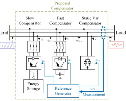
Proposed Compensator Control References
The method proposed in this dissertation for the compensation of non-periodic
load provides control references for three co-located devices, each corresponding to
one moving calculation window and one decomposed part of the compensated current.
These compensators are slow compensator with high power rating, large calculation
window, and low switching frequency; fast compensator with lower power rating,
shorter calculation window, and higher switching frequency; and the reactive
com-pensator which is an ordinary static VAR comcom-pensator (SVC). In this chapter, the
structure of this proposed control reference is discussed. Moreover, a new structure
is proposed to share the bandwidth and rating between the compensators.
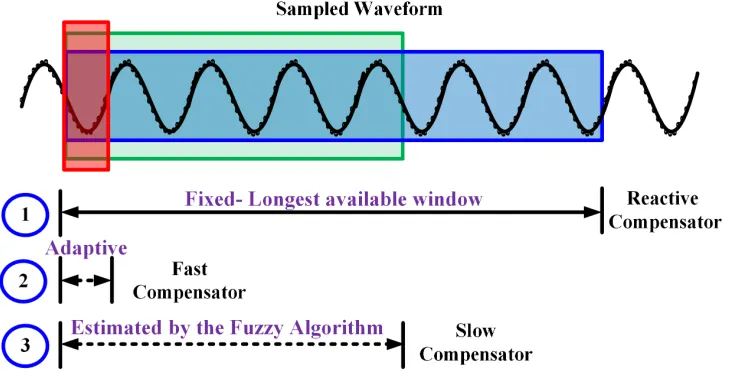
The complete structure of the compensator with these three compensation devices
are shown in fig. 3.2. Each one of the proposed devices has a particular moving
window for the calculation of their current reference. The fast compensator window
length is a short fraction of the generated voltage frequency period which results in
higher compensation speed compared to other non-periodic compensation techniques,
which use windows equal or larger than the fundamental frequency period of the
generated voltage. For example, in [48], a window length equal to ten times the period
of the fundamental frequency of the voltage is chosen. The reactive compensator
window length is one cycle of generated voltage frequency period. The window length
of the slow compensator is larger than the other two compensators since it is in
charge of the low-frequency part of the non-periodic current. Therefore, to ideally
[42]. However, since such design is not realizable, the proposed algorithm uses an
adaptive fuzzy algorithm to look for optimized window length. The optimized window
is found in a way that the power quality requirements are met while having the
minimum energy storage size for the slow compensator. The tri-window structure of
the proposed method is shown in fig. 3.1.
Figure 3.1: The tri-window structure of the proposed method.
3.1
Reactive Compensator
In order to eliminate the reactive current, a Static VAR Compensator is used. The
reference current for this compensator is calculated using the following equations:
q(t) =v(t−T0
4 )(i(t)−iF C(t)) (3.1)
Q(t) = 1
T0
Z t+T0
t
q(τ)dτ (3.2)
Be=
Q V12
(3.3)
iR1(t) = Bev(t−
T0
4 ) (3.4)
Figure 3.2: Structure of the proposed compensator.
where q is called instantaneous reactive power, Q is reactive power of the load, T0
is the period of one cycle of power frequency, Be is the equivalent susceptance, V1 is
the RMS value of the fundamental voltage, iR is the reactive current reference,and
iRemRC is the remaining current after the reactive compensation that will be loaded
to the fast compensator.
3.2
Fast Compensator
Passive filters prove ineffective in the compensation of loads with non-periodic
cur-rent since the inter-harmonic noise would coincide with their resonant frequencies.
Therefore, active filters are required to filter out the high-frequency and low-frequency
refer-ence is proposed in this dissertation for the compensation of high-frequency content
of the current. The main purpose of this compensator is to make sure that the
com-pensator with the large rating (slow comcom-pensator) does not require high bandwidth.
Therefore, this compensator is responsible for conditioning the current waveform to
a bandwidth level that is manageable by the slow compensator.
The reference current of the fast compensator is calculated using the following set
of equations:
pF C(t) =v(t)iRemRC(t) (3.6)
PF C(t) =
1
kT0
Z t+kT0
t
pF C(τ)dτ (3.7)
VF C2(t) =
1
kT0
Z t+kT0
t
v(τ)2dτ (3.8)
GeF C(t) =
PF C(t)
VF C2(t)
(3.9)
iF C(t) =iRemRC(t)−GeF Cv(t) (3.10)
iRemF C(t) =iRemF C(t)−iF C(t) (3.11)
wherepF C is instantaneous power of the load after reactive compensation, PF C is the
power average over a window length which is equal to the fraction of supply voltage
period (kT0),VF C2 is the voltage RMS calculated over the same window length (kT0),
GeF C is the equivalent conductance of the load after reactive compensation over the
same window length (kT0), iF C is the reference current of the fast compensator, and
iRemF C is the remaining current after the fast compensation.
The final purpose of any compensation is to achieve a constant equivalent
conduc-tance. However, such goal requires an active filter with very high rating, large energy
storage, and large bandwidth. In this dissertation, the purpose of the fast
compen-sator is to compensate the low power-high frequency part of the current waveform.
This goal is achieved through adaptively controlling the fast compensator window
In general the load equivalent conductance seen by the fast compensator could be
written as follows:
GeF C(t) =
P +peLF(t) +peHF(t)
V2 +vf2LF(t) +vf2HF(t)
(3.12)
where symbols “˜00and “¯00demonstrate time-varying and constant quantities,
respec-tively, and subscript “LF00 and “HF00 demonstrate low frequency and high frequency
components, respectively.
The constant equivalent conductance is achievable when both nominator and
de-nominator have zero time-varying components. For such purpose, two moving
aver-age FIR (finite impulse response) filters (equations (3.8) and (3.9)) are used in Fryze
power theory. However, the basic Fryze power theory based compensator (k = 1)
does not allow for adaptive sharing of the bandwidth between compensators and also
compensation of non-periodic current.
3.3
Slow Compensator
The non-periodic part of the current has theoretically infinity large period [42].
Therefore, the higher compensation window results in smoother compensation and
higher power quality. The existing attitude for non-periodic compensation in the
literature is that, the longer the window size, the better the compensation quality.
Though it is correct in general, the longer window also implies longer transient
re-sponse. Therefore, by choosing possibly a smaller window (with similar power quality
of longer windows) the transient time after a load change could be minimized without
compromising the power quality. Moreover, by decreasing the window length size,
the required bandwidth of the slow compensator is decreased.
Therefore, in order to remove the non-periodic and low frequency part of the
current, an active filter, whose window length is adaptively modified is designed.
modulation index. The slow compensator current is calculated using the following
relations:
p(t) = v(t)iRemF C(t) (3.13)
P(t) = 1
T
Z t+T
t
p(τ)dτ (3.14)
Ge1 =
P V12
(3.15)
iSC(t) =iRemF C(t)−Ge1(t)v1(t) (3.16)
where Ge1 is the total power equivalent conductance of the fundamental frequency
which reflects the equivalent conductance of the load in case all the current is being
transferred with the fundamental frequency, iSC is the current being compensated by
the slow compensator, and T is the window length for the calculation of equivalent
conductance.
The ultimate goal of the slow compensator is to achieve the equivalent conductance
with zero oscillation. However, in the practical case, such goal is not achievable since
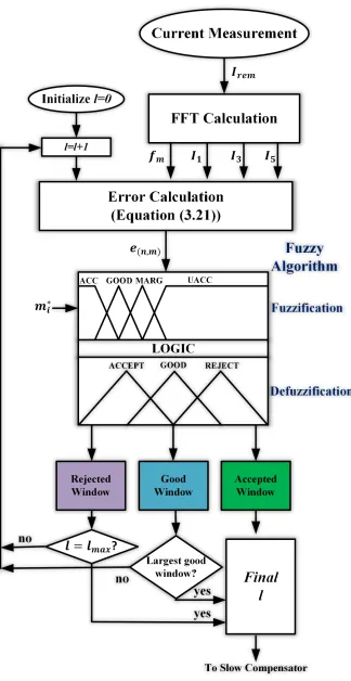
it requires an infinitely large energy storage. In this work, a fuzzy-based algorithm is
proposed to minimize the oscillating part of the equivalent conductance by adaptively
modifying the length of the calculation window:
Ge(t) =Ge1(t) +Gee(t) (3.17)
where Ge(t) is the measured load equivalent conductance and Gee is the oscillating
part of the equivalent conductance. The goal of the slow compensator is to achieve
constant Ge1, and therefore zeroGee(t).
It could be proven that for a non-periodic current, the oscillating part of the
e
Ge ∝
sin(2πlq)
l (3.18)
f or l = T
T0
(3.19)
f or q=±mk (3.20)
where n is the order of existing harmonics in the current (odd numbers for power
systems),mis the order of existing harmonics in the modulating signals (odd numbers
for regular modulating signals), k is the modulation ratio (∆ωω
0), ∆ω(= 2πfm) is the modulation frequency, andω0is the power system frequency. Please see the Appendix
B for detailed mathematical explanation.
It could be concluded that in order to reach zero oscillating conductance (pure
sinusoid current), one of two requirements shall be met; (1) infinite window length
(1/T = 0), and (2) integer 2lq (cos(2πlq) = 0) . Though the former is unrealizable
(infinite energy storage is needed), the latter could be realized using a
minimiza-tion algorithm in a way that the window length (l) is to be manipulated to reach a
minimized error signal e(n, m, l):
e(n, m, l) = 2lq−round(2lq), f or n= 3,5, .., m= 1,3, ... (3.21)
However, it is not feasible to minimize all the errors with one particular window
(l). Therefore, an algorithm is needed that incorporates the importance of each
current harmonics and modulation harmonic (n, m) in finding the best window size.
The flowchart of the proposed Mamdani-based fuzzy algorithm part of the slow
compensator is shown in fig. 3.3. The method uses FFT calculation of the remainder
current (irem = iL−iF −iR) to find the dominant harmonics, the modulation
fre-quency (∆ω), and modulation ratio (k). Using FFT for such purpose results in less
computational burden compared to other methods such as Kalman filtering used in