The Effect of Professional Development on Middle School Teachers' Technology Integration: An Action Research Study

(1)

University of South Carolina

Scholar Commons

Theses and Dissertations

5-2017

Dynamic Model and Control of Quadrotor in the

Presence of Uncertainties

Courage Agho

University of South Carolina

Follow this and additional works at:https://scholarcommons.sc.edu/etd Part of theElectrical and Computer Engineering Commons

This Open Access Thesis is brought to you by Scholar Commons. It has been accepted for inclusion in Theses and Dissertations by an authorized administrator of Scholar Commons. For more information, please [email protected].

Recommended Citation

(2)

DYNAMIC MODEL AND CONTROL OF QUADROTOR IN THE

PRESENCE OF UNCERTAINTIES

by Courage Agho Bachelor of Science

University of South Carolina, 2015

_________________________________________________ Submitted in Partial Fulfillment of the Requirements

For the Degree of Master of Science in Electrical Engineering

College of Engineering and Computing University of South Carolina

2017 Accepted by:

Xiaofeng Wang, Director of Thesis Bin Zhang, Reader

(3)

ii

(4)

iii

ACKNOWLEDGMENTS

(5)

iv

ABSTRACT

This thesis considers the control of quadrotor using a linear PID control and ℒ₁

adaptive control. In a justifiable concept, PID controller can be used to control a quadrotor, but in the presence of uncertainties or disturbance, the quadrotor can’t be automatically adjusted to control the changing dynamics of the quadrotor. To solve the problem associated with uncertainties, various control methodology can be used for controlling the changing dynamic of quadrotor, but in this thesis, ℒ₁ adaptive control is used because it allows for fast and robust adaptation for desired transient performance in the presence of matched and unmatched uncertainties.

In this thesis, we would derive the quadrotor model which gives us an access on how we can track positions, then design a controller to track these desired positions using PID control. Same concept used for PID control would be used for ℒ1 adaptive control in

(6)

v

LIST OF FIGURES

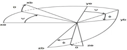
Figure 2.1: Body and Earth Frame with their Corresponding Angle …………..…..……..3

Figure 2.2: Movement around Angles on the Coordinates System because of Force ………..……….5

Figure 3.1: Moment acting on the Quadcopter ………...………..……...7

Figure 4.1: Altitude Position Tracking Using PID Controller [Z-Axis] ……..………...13

Figure 4.2: Block Diagram for Translational Control ………..………....14

Figure 4.3: Roll Position Tracking Using PID Controller [X-Axis] ………..………..….14

Figure 4.4: Pitch Position Tracking Using PID Controller [Y-Axis] ………..……...14

Figure 4.5: Yaw Angle Tracking Using PID Controller [Z-Axis] …………..…………..15

Figure 4.6: Controller Gain Constant ……….…………..…….15

Figure 4.7: Altitude Response to Step Input Disturbance ………..……..………...16

Figure 5.1: Closed Loop Architecture for Direct MRAC ………..………...18

Figure 5.2: Closed Loop Architecture for Indirect MRAC ………..…………....….19

Figure 5.3: Closed Loop Architecture for ℒ₁ Adaptive controller …………..………...21

Figure 5.5: Altitude Position Using State Feedback Control [Z-Axis] …………...……23

Figure 5.6: State Feedback for Altitude Control ………..…….….……...24

Figure 5.7: Altitude Position Tracking with Response to Varying Uncertainties and Extra Mass [Z-Axis]………..………....26

(9)

viii

Figure 5.9: Estimate Uncertainty vs Real Uncertainty for Altitude Control …...…...26

Figure 5.10: Yaw Angle Tracking Using State Feedback Control.………...27

Figure 5.11: Tracking of Desired Reference Yaw Angle with Varying Input Uncertainties ………...…...…...29

Figure 5.12: Estimated Uncertainty vs Real Uncertainty for Yaw Control …………...29

Figure 5.13: State Feedback Design in Simulink ………..…31

Figure 5.14: Roll Position Tracking without Varying Input Uncertainties ………..31

Figure 5.15: Pitch Angle at a Desired Position of 1.4m ………...32

Figure 5:16 Pitch Angle at a Desired Position of 25m ………...32

Figure 5.17: Pitch Angle with Desired Position of 25m ………..……….33

Figure 5.18: Pitch Angle with Desired Position of 1.4m ………..…33

Figure 5.19: Tracking of Desired Position of 1.4m with Pitch Angle Limitation ...34

Figure 5.20: Tracking of Desired Position of 25m with Pitch Angle Limitation ...34

Figure 5.21: Roll Position Tracking with Varying Matched and Unmatched Uncertainties without Compensation for Unmatched Uncertainties ...36

Figure 5.22: Roll Position Tracking with Varying Matched Uncertainties ....…..…..…..37

Figure 5.23: Structural Design for Roll Control ………...37

Figure 5.24: Estimate Uncertainty vs Real Uncertainty for Roll Control ...37

Figure 5.25: Estimate Uncertainty vs Real Uncertainty for Unmatched Uncertainties Roll Control ...38

Figure 5.26: Roll Position Tracking with Varying Matched and Unmatched Uncertainties ………...………..………....38

Figure 5.27: Feedback Response without Disturbance ……..…...39

(10)

ix

Uncertainties Pitch Control ………..………...……...39

Figure 5.30: Estimate Uncertainty vs Real Uncertainty for Unmatched Uncertainties Pitch Control ………...………..…...……..40

Figure 6.1: Disturbance Limit ………...41

Figure 6.2: Altitude Position Tracking Using ℒ1 Adaptive Controller [Z-Axis] ...42

Figure 6.3: Yaw Position Tracking Using ℒ1 Adaptive Controller [Z-Axis] ………..….42

Figure 6.4: Roll Position Tracking Using ℒ₁ Adaptive Controller [X-Axis] …...42

Figure 6.5: Pitch Position Tracking Using ℒ₁ Adaptive Controller [Y-Axis] …...43

Figure 6.6: Simulink Design with Uncertainties Input ………...……..………..…..43

(11)

1

CHAPTER 1 INTRODUCTION

In recent year, research on quadrotors has become popular, but the first quadrotor was built in 1907 by Louis Charles Bréguet. Helicopter development was desired over quadrotor, but with recent progress in technological development, more funds and time has been dedicated to the research of quadrotors. Quadrotor became popular because helicopter uses tail rotors to counterbalance the torque or rotating forces generated by the single main rotor. Because of the counterbalancing tail rotor, it inefficient in term of control, power consumption and cost production. Due to the work of Charles Richet and Dr George de Bothezat in 1956, propellers where used to control the quadcopter roll, pitch and yaw angle. In addition to those improvements, technological advancement in batteries weight, life and density has greatly helped the research of quadrotors. Recent development in processors and low cost efficient sensors has greatly impacted quadrotor development as well.

(12)

2

This thesis focuses on creating an accurate control mechanism to achieve stabilized flight control using ℒ₁ adaptive control because it mitigates the issues of uncertainties and disturbance.

A quadrotor is a nonlinear system device and control for nonlinear system is complex because we desire a system that has fast adaptation and response in real time and robust enough to mitigate the issue of disturbance and uncertainties. Adaptive control was developed as a technique for automatic adjustment in real time. To achieve and maintain desired system performance, the aerospace industries and institution started research on adaptive controller and today it is used widely by different industries and for different purposed. Model reference adaptive control (MRAC) is a type of adaptive control and ℒ₁ adaptive control is a further use of model reference adaptive control (MRAC). Apart from canceling of uncertainties and disturbance, ℒ1 adaptive control theory has architecture in

(13)

3

CHAPTER 2 QUADROTOR STRUCTURE

2.1 QUADCOPTER COORDINATE SYSTEM

A quad employs different control mechanism such as roll, pitch, and yaw which in most cases are represented by angle of rotation around the center of the quad craft. These angles make up for the control of the altitude of the quadcopter and to track the altitude of the quadcopter, a two-coordinate system is required. There is the body frame system which is attached to the quad at its center of gravity and the earth frame system which is fixed to the earth and it is sometimes refer to as an inertial coordinate system. The angular different between the two coordinate helps define the behavior of the quad altitude in space. The attitude system can be derived by rotating the body frame around the z axis of the earth frame by the yaw angle 𝜑, which is tend followed by rotating around the y-axis by the pitch angle 𝜙 and finally by rotating around the x-axis by the roll angle 𝜃. This is shown in figure 2.1 as well as its rotation matrix that has the body and earth frame parallel to each other and their sequence of rotation is known as the Z-Y-X rotation and its rotation matrix is shown in equation 2.1.

(14)

4

𝑅 = [

cos(𝜃) sin (ψ) sin(ϕ) sin(𝜃) cos(ψ) cos(ϕ) sin(𝜃) cos(ψ) + sin(ϕ) sin (ψ) cos(𝜃) sin (ψ) sin(ϕ) sin(𝜃) sin(ψ) + cos(𝜃) cos (ψ) cos(ϕ) sin(𝜃) sin(ψ) − sin(𝜃) cos (ψ)

−sin (𝜃) sin(ϕ) cos (𝜃) cos(ϕ) cos (𝜃)

] (2.1)

2.2 STATES OF THE QUADCOPTER

From the section of coordinate system, the angle of roll, pitch, and yaw are represented as 𝜙, 𝜃, 𝜓 in addition to their angle, angular velocity is also required and can be represented as 𝜙̇, 𝜃̇, 𝜓̇ these are the first six state of the quadcopter that shows a relationship between the quadcopter and the earth coordinate system. The next six states show a physical relationship of the physical location within the earth fixed system and it is denoted as 𝑋, 𝑌, 𝑍. In addition to their physical position is their quad velocity along these axes and it is denoted as 𝑋,̇ 𝑌,̇ 𝑍̇. Together they make up the 12 states of the quadcopter and as shown below.

2.3 HOW QUADROTOR WORKS

(15)

5

and yaw is possible. The diagram in figure 2.2 shows how the force generated by each motor affects a change the direction of the quadcopter along the angles on the coordinate system

(16)

6

CHAPTER 3 DYNAMIC MODEL

The dynamic model of a quadcopter is a subsystem that is divided into two subsystems known as the rotational subsystem that represent (roll angle, pitch angle and yaw angle) and translational subsystem that represent (Z position, X position, Y position). The rotational side of the Quadcopter is completely actuated while the translational side of the subsystem is under actuated

3.1 MOMENT ACTION ON THE QUADROTOR

An effect of rotation is the force generated called aerodynamic force and moment generated called aerodynamic moment. The aerodynamic moment is the combination of aerodynamic force multiplied by its distance. It is dependent on the geometry of the propeller and by identifying the moment and force generated by the propeller, we can understand the moment acting on the quadcopter. From figure 3.1, when F2 is multiplied by the moment arm, a negative moment is generated about the y-axis. Using the same concept, F4 generates a positive moment and the total moment about the x-axis can be expresses as

𝑀_𝑋 = (𝐹4 − 𝐹2)𝑙 (3.1)

Same concept is applied for My Where

(17)

7

For the moment about the Z axis, the thrust of the rotor does not cause a moment, but rather the rotor rotation in relation with the rotor speed causes a moment and is represented as

𝑀𝑧 = (𝐹1 + 𝐹3 − 𝐹2 − 𝐹4)𝑙𝑐 (3.3)

Where c gives the relationship between the rotor speed and its effect on the quadrotor rotation about the body frame and the combination of each body frame axis gives us a matrix as shown below.

𝑀𝑏 = [

(𝐹4 − 𝐹2)𝑙 (𝐹1 − 𝐹3)𝑙 (𝐹1 + 𝐹3 − 𝐹2 − 𝐹4)𝑙𝑐

] (3.4)

Figure 3.1: Moment acting on the Quadcopter 3.2 INERTIAL MATRIX

The inertial matrix for a quadcopter is a diagonal matrix as shown below. The structure of the matrix is because quadcopters are built symmetrically with respect to the coordinate systems that were explained in section 2.1.

𝐽 = [

𝐽𝑥 0 0

0 𝐽_𝑦 0

0 0 𝐽𝑧

] (3.5)

From the matrix above 𝐽_𝑥, 𝐽_𝑦 and 𝐽_𝑧 are the area moments of inertia about the principle axes on the body frame.

(18)

8

The control input is from the controller and the input to a quadcopter is from the force generation by the motor, and for simplicity, Control Input Vector (U) can represent Force (F) where

𝑈_𝑡𝑧 = (𝐹1 + 𝐹2 + 𝐹3 + 𝐹4) (3.6)

𝑈_𝑡𝑥 = (𝐹4 − 𝐹2) (3.7)

𝑈𝑡𝑦 = (𝐹1 − 𝐹3) (3.8)

𝑈_𝑟𝑧= (𝐹1 + 𝐹3 − 𝐹2 − 𝐹4) (3.9)

From equation 3.4, the moment acting on the quadcopter in its body frame can be represented as

[ 𝑈_𝑡𝑥𝑙 𝑈_𝑡𝑦𝑙 𝑈_𝑟𝑧𝑙𝑐

] (3.10)

3.4 ROTATIONAL SUBSYSTEM

The rotational part of the quadcopter is derived from the concept of rotational equation of motion and by using Newton-Euler method derived from the body frame of the quadcopter with a generalized formula as shown below.

𝑀_𝑏 = (𝐽𝑤̇ + 𝑤×𝑗𝑤 + 𝑀_𝑔) (3.11)

Where: 𝐽 represents quadrotor inertia Matrix, 𝑤 represents angular velocity, 𝑀_𝑔represents the gyroscopic moment generated due to its rotor inertial and 𝑀_𝑏 represents moments acting on the quadcopter in its body frame. For simplicity, the gyroscopic moment would not be considered because the inertial generated by the quadcopter is much larger that the inertial generated by the rotor. So, our final rotor equation would be

𝑀_𝑏 = (𝐽𝑤̇ + 𝑤×𝑗𝑤) (3.12)

(19)

9 [ 𝑈_𝑡𝑥𝑙 𝑈𝑡𝑦𝑙 𝑈_𝑟𝑧𝑙𝑐 ] = [

𝐽𝑥 0 0

0 𝐽_𝑦 0

0 0 𝐽_𝑧

] [ 𝜙̈ 𝜃̈ 𝜓̈ ] + [ 𝜙̇ 𝜃̇ 𝜓̇ ] × [

𝐽𝑥 0 0

0 𝐽_𝑦 0

0 0 𝐽_𝑧

] [ 𝜙̇ 𝜃̇ 𝜓̇ ]

When the matrix is rewritten to have its angular acceleration, we would have

𝜙 ̈ = 𝑙 𝐽_𝑥𝑈𝑡𝑥+

𝐽_𝑦 𝐽_𝑥𝜓̇𝜃̇ −

𝐽_𝑧

𝐽_𝑥𝜃̇𝜓̇ (3.13)

𝜃̈ = 𝑙

𝐽_𝑦𝑈𝑡𝑦+ 𝐽_𝑧 𝐽_𝑦𝜓̇𝜙̇ −

𝐽_𝑥

𝐽_𝑦𝜙̇𝜓̇ (3.14)

𝜓̈ = 𝑙𝑐 𝐽_𝑧𝑈𝑟𝑧+

𝐽_𝑥 𝐽_𝑧𝜃̇𝜙̇ −

𝐽𝑦

𝐽_𝑧𝜙̇𝜃̇ (3.15)

3.5 TRANSLATION SUBSYSTEM

The translation subsystem is based on translational equation of motion and it is based on newton second law which is derived from the earth inertial frame and it is presented in the format below.

𝑚𝑑̈ = [ 0 0 𝑚𝑔

] + 𝑅×𝐹_𝑛𝑔 (3.16)

Where: m is the mass, g is gravitational acceleration, 𝐹_𝑛𝑔 is non-gravitational force which is the physical location within the earth fixed system and R is the rotational matrix. 𝐹_𝑛𝑔 is shown in equation 3.17. It is the addition of all the thrust force produced by the four propellers and the negative sign is because the thrust force generated is acting upward while the z-axis of the body frame is point down. R is for the rotational matrix that is generated to transform the forces generated from the body frame to the earth frame. By substitution and simplification, we would derive the acceleration along the X, Y, and Z axis.

𝐹_𝑛𝑔= [ 0 0 −𝑈_𝑡𝑧

(20)

10

By substitution of these equations into equation 3.16, we would get

𝑚 [𝑋̈𝑌̈ 𝑍̈

] = [ 0 0 𝑚𝑔

] + [

cos(𝜃) sin (ψ) sin(ϕ) sin(𝜃) cos 𝜓 − cos(ϕ) sin(𝜃) cos(ψ) + sin(ϕ) sin (ψ) cos(𝜃) sin (ψ) sin(ϕ) sin(𝜃) sin(φ) + cos(𝜃) cos (ψ) cos(ϕ) sin(𝜃) sin(ψ) − sin(𝜃) cos (ψ)

−sin (𝜃) sin(ϕ) cos (𝜃) cos(ϕ) cos (𝜃)

] × [ 0 0 −𝑈𝑡𝑧

]

When the matrix is rewritten to have its acceleration, we would have

𝑋̈ = −𝑈𝑡𝑧

𝑚 (− cos(𝜙) sin(𝜃) cos(𝜓) + sin(𝜙) sin(𝜓)) (3.18)

𝑌̈ = −𝑈𝑡𝑧

𝑚 (cos(𝜙) sin(𝜃)sin(𝜓) + sin(𝜃) cos(𝜓)) (3.19)

𝑍̈ = −𝑈𝑡𝑧

𝑚 (cos(𝜙) cos(𝜃)) − 𝑔 (3.20)

The quadrotor parameter are defined below and these parameters would be use for simulation

𝑚 = 0.8𝑘𝑔; 𝑙 = 0.25𝑚; 𝑔 = 9.81 𝑁

𝑘𝑔; 𝑐 = 0.02; 𝐽𝑥 = 𝐽𝑦 = 0.015𝑘𝑔𝑚 2_;_𝐽

(21)

11

CHAPTER 4 CONTROL OF THE QUADROTOR

Building a control system to control how the quadcopter operate is very important. The dynamic model of the quadcopter is an open loop and closed loop control is a preferred method for any design because the system records the output instead of the input and modifies its output per a preferred condition. For successful maneuvering of the quadcopter, we need 4 controllers that would be designed to act as in input to the model of the quadcopter. These 4 controllers represent the 4-input coming from the transmitter assuming this was a physical quadcopter. They are throttle, roll, pitch, and yaw input. The throttle coming from the transmitter can be represented and called the altitude controller or translational controller in the z axis. The roll, pitch, and yaw input from the transmitter can be called rotational controller that is dependent on the angle ϕ, θ, 𝜑. The translational subsystem of the model is partially dependent on the rotational subsystem because it is under-actuated.

(22)

12

𝑍̈ = 1

𝑚(−𝑈𝑡𝑧) (4.1)

𝑋̈ = −1

𝑚𝜃(𝑈𝑡𝑧) (4.2)

𝑌̈ = 1

𝑚𝜙(𝑈𝑡𝑧) (4.3)

𝜓̈ = 𝑙

𝐽_𝑧𝑈𝑟𝑧 (4.4)

𝜃̈ = 𝑙 𝐽𝑦

𝑈𝑡𝑥 (4.5)

𝜙̈ = 𝑙 𝐽𝑋

𝑈𝑡𝑦 (4.6)

4.1 TRANSLATION CONTROL ALONG THE Z AXIS

The translational controller takes an error signal as an input which is the difference between the actual altitude and desired altitude and produces a control signal 𝑈_𝑡𝑧. The control signal 𝑈_𝑡𝑧is responsible for the altitude of the quadcopter and mathematical equation is shown below. The equation below uses the concept of a PID controller and for simulation of result, we would multiply the input data by (-1) to compensate for the negative sign in equation 4.1 and the controller response to the closed loop simulation is shown in figure 4.1.

𝑈_𝑡𝑧 = 𝐾𝑝(𝑧 − 𝑧𝑑) + 𝐾𝑖 ∫(𝑧 − 𝑧𝑑) + 𝐾𝑑𝑑𝑧

(23)

13

Figure 4.1: Altitude Position Tracking Using PID Controller [Z-Axis] 4.2 TRANSLATION CONTROL ALONG THE X AXIS

The translational controller takes an error signal as an input which is the difference between the actual roll angle and the desired roll angle to produce a control signal 𝑈_𝑡𝑥. The control signal 𝑈_𝑡𝑥 is responsible for moving the quadcopter left and right about the X axis. The mathematical equation is shown below. The equation below uses the concept of a PID controller and because translation along the X axis is dependent on 𝜃, control of its desired position is not under a direct control.

𝑈_𝑡𝑥 = 𝐾𝑝(𝑥 − 𝑥𝑑) + 𝐾𝑖 ∫(𝑥 − 𝑥𝑑) + 𝐾𝑑𝑑𝑧

𝑑𝑡(𝑥 − 𝑥𝑑) (4.8)

This is because the X positions are under the translational subsystem which is under-actuated. To compensate for the under actuation of the system, the pitch angle can be used to control desired X position.

We would assume 𝑈𝑡𝑧 = 𝑚𝑔 which would cause loss in precision, but it also simplifies the

model for easier control. Equation 4.2 is then simplified as

𝑋̈ = −𝜃𝑔 (4.9)

(24)

14

negative sign in equation 4.2 and the controller response to the closed loop simulation is shown in figure 4.5.

Figure 4.2: Block Diagram for Translational Control

Figure 4.3: Roll Position Tracking Using PID Controller [X-Axis] 4.3 TRANSLATION CONTROL ALONG THE Y AXIS

𝑌̈ = 𝜙𝑔 (4.10)

The design for controller movement along the Y axis is design in similar method for translation along the X axis. The only difference is the Y axis is dependent on the roll angle.

(25)

15

The yaw controller takes an error signal as an input which is the difference between the actual yaw angle and the desired yaw angle to produce a control signal 𝑈_𝑟𝑦and the mathematical equation is shown below. The equation below uses the concept of a PID controller and the block diagram represent how the close loop method of the yaw controller would look like.

𝑈𝑟𝑦 = 𝐾𝑝(𝜓 − 𝜓𝑑) + 𝐾𝑖 ∫(𝜓 − 𝜓𝑑) + 𝐾𝑑

𝑑𝑧

𝑑𝑡(𝜓 − 𝜓𝑑) (4.11)

Figure 4.5: Yaw Angle Tracking Using PID Controller [Z-Axis]

From the design concept above, 6 PID controllers were designed with Kp, Ki, and Kd gain derived. Where the controller design for translational control on the X and Y axis would have two PID controller and their gain constants are shown in figure 4.6.

Kp (gain) Ki (gain) Kd (gain)

Translation Control along the Z Axis 0.4001 0.01019 3.491

Translation Control along the Y Axis 0.0366 0.0008775 0.3392

Translation Control along the X Axis 0.0366 0.0008775 0.3392

Rotation Control along the Z Axis 0.21 0.01225 0.7997

Rotation Control along the Y Axis 1.553 0.8375 0.5677

Rotation Control along the X Axis 1.553 0.8375 0.5677

(26)

16

(27)

17

CHAPTER 5 ℒ

₁

ADAPTIVE CONTROL

As you can see from section 4, using a conventional linear controller work fine when there is no disturbance or uncertainty, but when disturbance is added to the system as shown in figure 4.10, the controller is not able to adapt fast enough to compensate for the additional error. The process of creating an adaptation mechanism leads to further insight to the concept of adaptive controller.

(28)

18

5.1 DIRECT & INDIRECT ADAPTIVE CONTROLLER

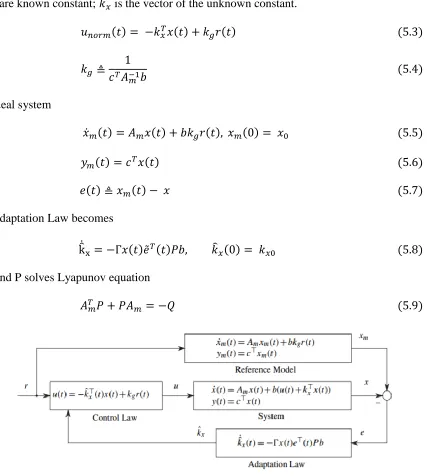
The architecture is shown in figure 5.1 and the differential equation of the real plant is

𝑥̇(𝑡) = 𝐴_𝑚𝑥(𝑡) + 𝑏(𝑢(𝑡) + 𝑘_𝑥𝑇𝑥(𝑡), 𝑥(0) = 𝑥₀ (5.1) 𝑦(𝑡) = 𝑐𝑇𝑥(𝑡) (5.2)

Where 𝐴_𝑚 defines matrix of the closed loop system, x(t) is the state of the system, b and c are known constant; 𝑘𝑥 is the vector of the unknown constant.

𝑢_{𝑛𝑜𝑟𝑚}(𝑡) = −𝑘𝑥𝑇𝑥(𝑡) + 𝑘𝑔𝑟(𝑡) (5.3)

𝑘_𝑔 ≜ 1

𝑐𝑇_𝐴 𝑚

−1_𝑏 (5.4)

Ideal system

𝑥̇𝑚(𝑡) = 𝐴𝑚𝑥(𝑡) + 𝑏𝑘𝑔𝑟(𝑡), 𝑥𝑚(0) = 𝑥0 (5.5)

𝑦_𝑚(𝑡) = 𝑐𝑇_{𝑥(𝑡) (5.6)}

𝑒(𝑡) ≜ 𝑥_𝑚(𝑡) − 𝑥 (5.7)

Adaptation Law becomes

k̂̇_x= −Γ𝑥(𝑡)𝑒̃𝑇(𝑡)𝑃𝑏, 𝑘̂_𝑥(0) = 𝑘_𝑥0 (5.8)

And P solves Lyapunov equation

𝐴_𝑚𝑇𝑃 + 𝑃𝐴_𝑚 = −𝑄 (5.9)

(29)

19

For stability test and analysis, Lyapunov function is used to test Lyapunov stability. By taking the first derivative of Lyapunov function, the signal stays bounded and the second derivative proves that the error converges when 𝑒(𝑡) ⟶ 0 𝑎𝑠 𝑡 ⟶ ∞ which in turns proves the application of Barbalat’s lemma equation on stability of time varying system. The theoretical approach used for direct MRAC is used as well for Indirect MRAC. The main difference is that the indirect method estimates the system parameters and the derivation of the adaptive law is independent of the control signal with its system architecture as shown in figure 5.2. The asymptotical convergence of its tracking error is also concluded using Barbalat’s lemma equation from Lyapunov stability and its adaptive law becomes

𝑘̂_𝑥= Γ𝑥(𝑡)𝑥̃𝑇_{(𝑡)𝑃𝑏, 𝑘̂}

𝑥(0) = 𝑘𝑥0 (5.10)

Figure 5.2: Closed Loop Architecture for Indirect MRAC 5.2 ℒ₁ ADAPTIVE CONTROLLER ARCHITECTURE

(30)

20

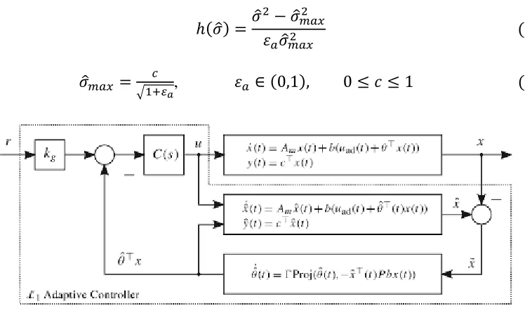
known as the ℒ1 adaptive controller is used. With ℒ1 adaptive controller, adaptation can be

separated from robustness. The architecture in figure 5.3 shows how ℒ1 adaptive controller is designed. The design approach is a combination of the MRAC state predictor and a low pass filter from the control input to the estimated model and the real plant. The controller compared to indirect MRAC is giving as

𝑢(𝑠) = 𝐶(𝑠)𝑛(𝑠) (5.11)

C(s) transfer function is bounded input-bounded output stable which is subjected to C(s)=1 with zero initialization. This is achievable with a first order low pass filter where

𝐶(𝑠) = ωc

𝑠+𝜔𝑐 (5.12)

and 𝜔𝑐 is the filter bandwidth, the filter should be chosen to maintain equation 5.13.

‖𝐺(𝑠)‖_ℒ1 <1

𝐿 (5.13)

Where

𝐺(𝑠) = 𝐻(𝑠)[1 − 𝐶(𝑠)], 𝐻(𝑠) = 𝑏

𝑠 + 𝑎𝑚

[1 − 𝐶(𝑠)] (5.14)

𝐿 ≜ 𝑚𝑎𝑥‖𝜃‖₁, 𝜃 ∈ Θ ⊂ ℝ𝑛_(5.15)

With low pass filter added to the system, robustness can be maintained with increased adaptation gain. The adaptation law for ℒ1 adaptive controller is giving by ΓProj(𝜃̂(𝑡), −𝑥̃𝑇_{(𝑡)𝑃𝐵𝑥(𝑡))}_{where the Proj operator ensures that the unknown parameter} 𝜃̂ stays bounded. 𝜃 would be replaced by 𝜎 for the quadrotor controller and the adaptive for ℒ1 adaptive controller is giving by ΓProj(𝜎̂(𝑡), −𝑥̃𝑇(𝑡)𝑃𝐵𝑥(𝑡)).

For projection operator with a given compact set{𝜎 ∈ ℝ | ‖𝜎‖ ≤ 𝑐},

Proj(𝜎̂, 𝜎̂′_{) =}_{𝜎̂′(1 − ℎ(𝜎̂)) 𝑖𝑓 (ℎ(𝜎̂) > 0 & 𝜎̂′ℎ(𝜎̂) > 0

(31)

21 Where

ℎ(𝜎̂) =𝜎̂ 2_{− 𝜎̂}

𝑚𝑎𝑥2

𝜀_𝑎𝜎̂_𝑚𝑎𝑥2 (5.17)

𝜎̂_𝑚𝑎𝑥 = 𝑐

√1+𝜀𝑎, 𝜀𝑎 ∈ (0,1), 0 ≤ 𝑐 ≤ 1 (5.18)

Figure 5.3: Closed Loop Architecture for ℒ₁ Adaptive controller 5.3 CONTROLLER DESIGN WITH ℒ₁ ADAPTIVE CONTROLLER

Just like is session 4, we would design four controllers to control the movement of the quadrotor using a state feedback approach. The information derived from the feedback approach would then be used to design an ℒ₁ adaptive controller to cancel out uncertainties. 5.4 TRANSLATION CONTROL ALONG THE Z-AXIS

From translation about the z axis,

𝑧̈ = 1

𝑚(cos(𝜙) cos(𝜃))(−𝑈𝑡𝑧) + 𝑔 (5.19)

𝑧̈ − 𝑔 = 1

𝑚(cos(𝜙) cos(𝜃))(−𝑈𝑡𝑧) (5.20)

𝑈𝑡𝑧 is the addition of the position control output and the control output for the cancelation

of gravity?

(32)

22

Since the quadrotor is moving about the z axis, 𝜃 and 𝜙 would be equal to zero. So

cos(𝜙) cos(𝜃) would be equal to 1. Therefore

𝑧̈ − 𝑔 = 1

𝑚(1) (−(𝑈𝑧𝑝+ 𝑈𝑧𝑔)) (5.22)

From equation 5.13, gravity would be ignored and later compensated where 𝑈_𝑧𝑔 is equal to mg. when it is ignored,

𝑧̈ = 1

𝑚(𝑈𝑧𝑝) (5.23)

State space equation

𝑥̇ = 𝐴_𝑧𝑝𝑥 + 𝐵_𝑧𝑝𝑈_𝑧𝑝

𝑦 = 𝐶𝑧𝑝𝑇 𝑥

[𝑧̇ 𝑧̈] = [

0 1 0 0] [

𝑧 𝑧̇] + [

0

1/𝑚] 𝑢; 𝑦 = [1 0] [ 𝑧

𝑧̇] (5.24)

With state feedback controller

𝑥̇ = 𝐴_𝑧𝑝𝑥 + 𝐵_𝑧𝑝𝑈_𝑧𝑝

𝑥̇ = 𝐴_𝑧𝑝𝑥 + 𝐵_𝑧𝑝(𝑘𝑔_𝑟− 𝑘𝑚_𝑧𝑝𝑇 𝑥) (5.25)

where kgr is the reference gain and kmzT = [k1tz k2tz]T which is the feedback gain.

Therefore

𝑥̇ = (𝐴𝑧𝑝− 𝐵𝑧𝑝𝑘𝑚𝑧𝑝𝑇 )𝑥 + 𝐵𝑝𝑘𝑔𝑟 (5.26)

Where 𝐴_𝑚_𝑧𝑝 = (𝐴_𝑃 − 𝐵_𝑝𝑘𝑚_𝑧𝑝𝑇 ₎_{So, the state spaces become} 𝑥̇ = 𝐴_{𝑚,𝑧𝑝}𝑥 + 𝐵𝑝𝑘𝑔𝑟

This changes the state space model to

[𝑧̇ 𝑧̈] = [

0 1

−𝑘1_𝑧(1

𝑚) −𝑘2𝑧(

1 𝑚) ] [𝑧_𝑧̇] + [ 0 1 𝑚

(33)

23 Transfer function of the state space model becomes

𝐺_𝑝(𝑠) =

1 𝑚 𝑠2_{+ 𝑘2}

𝑧(_{𝑚) 𝑠 + 𝑘1}1 𝑧(_𝑚)1

(5.28)

Compare to a reference transfer function

𝐺𝑟𝑒𝑓(𝑠) =

𝜔_𝑛2 𝑠2_{+ 2𝜁𝜔}

𝑛𝑠 + 𝜔𝑛2

(5.29)

From equation 5.23, 𝜔𝑛2 = 1/𝑚 and for critical damping, 𝜁 = 1. 𝑘1𝑡𝑧 = 1 and 𝑘2𝑡𝑧 = 2𝜁𝜔𝑛 𝑘2𝑡𝑧 = 2√𝑚 (5.30)

Therefore 𝑘2𝑡𝑧 = 1.79, where 𝑚=0.8. 𝑈𝑡𝑧 the controller output would be determined as 𝑈_𝑡𝑧 = (𝑘𝑔_𝑟+ 𝑘1_𝑧𝑧 + 𝑘2_𝑧𝑧̇ + 𝑚𝑔) (5.31)

Figure 5.5 is the simulation result tracking desired reference position and figure 5.6 is the Simulink design for control using state feedback.

(34)

24

Figure 5.6: State feedback for Altitude Control

With the feedback controller designed to ensure stable flight, we would then design a controller to cancel out uncertainties which is dependent on the adaptation law for uncertainty prediction. From equation 5.27, the state space model of the closed loop system is defined below.

𝐴𝑚,𝑧𝑝 = [

0 1

−𝑘1_𝑧(1

𝑚) −𝑘2𝑧( 1 𝑚)

] = [ 0 1

−1.25 −2.24] (5.32)

𝐵𝑝 = [ 0 1 𝑚

] (5.33)

For the adaptive law, we first need to determine the P matrix that will satisfy Lyapunov equation 𝐴_𝑚𝑇𝑃 + 𝑃𝐴_𝑚 = −𝑄. In order to achieve that, we would set Q as an identity matrix as shown below.

𝑄 = [1 0

0 1] (5.34)

𝑃 = [1.30 0.50

0.50 0.50] (5.35)

Adaptation control law

θ̂̇ = ΓProj(𝜎̂(𝑡), −𝑥̃𝑇_{(𝑡)𝑃𝐵𝑥(𝑡)) (5.36)}

θ̂̇ = ΓProj(𝜎̂(𝑡), − [𝑧̃ 𝑧̃̇] [

1.30 0.50 0.50 0.50] [

0 1 𝑚

]) (5.37)

θ̂̇ = ΓProj(𝜎̂(𝑡), −(0.63𝑧̃ + 0.63𝑧̃̇)) (5.38)

𝐺ℒ1,𝑡𝑧 = [[𝑠𝐼 − 𝐴𝑚,𝑝]

−1

𝐵𝑝] [1 − 𝐶𝑡,𝑧(𝑠)] (5.39)

(35)

25

𝐺_{ℒ1,𝑡𝑧} =

[

1.25𝑠

𝑠3_{+ 102.24𝑠}2_{+ 225.25𝑠 + 125} 1.25𝑠2

𝑠3_{+ 102.24𝑠}2_{+ 225.25𝑠 + 125]}

(5.40)

‖𝐺ℒ1,𝑡𝑧‖_ℒ1= 0.003 which give us an uncertainty limit of 333.33N. with that, the

adaptation gain can be big enough for faster adaptation. Also from equation 5.38, 𝑧̃ = 𝑧̂ − 𝑧 and 𝑧̃̇ = 𝑧̂̇ − 𝑧̇. For simulation, a varying uncertainty of -10N to 10N would be used with an adaptation gain of 10000. Figure 5.7 is the simulation result tracking desired reference position using ℒ₁ adaptive controller. Figure 5.8 shows the structural design of the altitude controller in Simulink and figure 5.9 shows the simulation of the estimated uncertainty vs the real uncertainty.

Another external force that could affect quadrotor movement in the Z axis is the input of extra mass. Theoretically, there is no limit on the amount of extra mass that a quadrotor can lift, but with a physical system, the amount of thrust and rotor speeds are limited. Most physical quadrotor are designed so that the sum of all four motors can lift at least twice its original mass. Assuming our simulation is designed for that purpose,

𝑚_{𝑒𝑥𝑡𝑟𝑎} ≤ 0.8. Therefore equation (5.23) can be rewritten as 𝑧̈ = 1

𝑚+𝑚𝑒𝑥𝑡𝑟𝑎(𝑈𝑧𝑝). Same

(36)

26

Figure 5.7: Altitude position [Z-Axis] with response to Varying Uncertainties and Extra Mass

5.8: Structural Design of the Altitude Controller

5.9: Estimate Uncertainty vs Real Uncertainty for Altitude Control 5.5 ROTATION CONTROL ABOUT THE Z-AXIS

(37)

27

𝜓̈ = 𝑙

𝐼_𝑧𝑧𝑈𝑟𝑧 (5.41)

State space feedback is

[𝜓̇ 𝜓̈] = [

0 1

−𝑘1_𝑟𝑧(𝑙𝑐

𝐽_𝑧) −𝑘2𝑟𝑧( 𝑙𝑐 𝐽_𝑧)

] [𝜓 𝜓̇] + [

0

𝑙𝑐/𝐽_𝑧] 𝑟𝑟𝑧 (5.42)

𝑦 = [1 0] [𝜓

𝜓̇] (5.43)

Transfer function is

𝐺_𝑟,𝑧(𝑠) =

𝑙𝑐 𝐽_𝑧

𝑠2 _{+ 𝑘2} 𝑟,𝑧(𝑙𝑐_𝐽

𝑧) 𝑠 + 𝑘1𝑟,𝑧( 𝑙𝑐 𝐽𝑧)

(5.44)

From equation 5.23, 𝜔_𝑛2₌𝑙𝑐

𝐽𝑧 and for critical damping, 𝜁 = 1. 𝑘1𝑟,𝑧 = 1 and 𝑘2𝑟,𝑧 = 2𝜁𝜔𝑛

𝑘2_𝑡,𝑥 = 2√𝑙𝑐

𝐽_𝑧 (5.45)

𝑘2_𝑟,𝑧 = 4 𝑤ℎ𝑒𝑟𝑒 𝑙 = 0.25𝑚, 𝑐 = 0.02, 𝐽_𝑧 = 0.02𝑘𝑔𝑚2

𝑈𝑟𝑧= 𝑟𝑟𝑧− 𝑘1𝑟,𝑧𝜓 − 𝑘2𝑟,𝑧𝜓̇ (5.46)

Figure 5.10: Yaw Angle Tracking Using State Feedback Control Where

𝐴_𝑚 = [

0 1

−𝑘1_𝑧(1

𝑚) −𝑘2𝑧(

1 𝑚)

] = [ 0 1

(38)

28

𝐵𝑚 = [ 0 𝑙𝑐 𝐽_𝑧

] (5.48)

For the adaptive law, we first need to determine the P matrix that will satisfy Lyapunov equation 𝐴_𝑚𝑇_{𝑃 + 𝑃𝐴}

𝑚 = −𝑄.

The P matrix to satisfy Lyapunov equation is

𝑃 = [4.50 0.50

0.50 0.625] (5.49)

θ̂̇ = ΓProj(𝜎̂(𝑡), −𝑥̃𝑇(𝑡)𝑃𝐵𝑥(𝑡)) (5.50)

θ̂̇ = ΓProj(𝜎̂(𝑡), − [𝜓̃ 𝜓̃̇] [

4.50 0.50

0.50 0.625] [ 0 𝑙𝑐 𝐽𝑧

]) (5.51)

θ̂̇ = ΓProj(𝜎̂(𝑡), − (0.125𝜓̃ + 0.156𝜓̃̇)) (5.52)

𝐺_{ℒ1,𝑟𝑧} = [[𝑠𝐼 − 𝐴_𝑚]−1_𝐵

𝑚][1 − 𝐶𝑟,𝑧(𝑠)] (5.53)

Using matlab, the transfer function is where wc =100 for the low pass filter

𝐺_{ℒ1,𝑟𝑧} =

[

0.25𝑠

𝑠3_{+ 101𝑠}2_{+ 100.25𝑠 + 25} 0.25𝑠2

𝑠3_{+ 101𝑠}2_{+ 100.25𝑠 + 25]}

(5.54)

‖𝐺_{ℒ1,𝑡𝑧}‖

ℒ1= 0.001 which give us an uncertainty limit of 1000N. With that, the adaptation

gain can be big enough for faster adaptation. Also from equation 5.52, 𝜓̃ = 𝜓̂ − 𝜓 and

𝜓̃̇ = 𝜓̂̇ − 𝜓̇. For simulation, a varying uncertainty of -10N to 10N would be used with an adaptation gain of 10000. Figure 5.11 provides result tracking desired reference angle using

(39)

29

Figure 5.11: Tracking of Desired Reference Yaw Angle with Varying Input Uncertainties

Figure 5.12: Estimated Uncertainty vs Real Uncertainty for Yaw Control 5.6 TRANSLATION CONTROL ALONG THE X-AXIS

(40)

30

small and does not have a huge effect on movement in the X and Y direction. Also, equation 5.55 can be linearized around hovering mode were 𝜙̇, 𝜃̇, 𝜑̇ is equal to zero.

𝜃̈ = 𝑙 𝐽𝑦

𝑈𝑡𝑥 (5.55)

̈

𝑋̈ = 1

𝑚(cos(𝜙) sin(𝜃) sin(𝜑) + sin(𝜃) 𝑠𝑖𝑛(𝜑)(−𝑈𝑡𝑧) (5.56)

Like the translational controller using small angle approximation,

𝑋̈ = −1

𝑚𝜃(𝑈𝑡𝑧) (5.57)

It is also important to note that when small angle approximation is used,

sin 𝜃 ≈ 𝜃

cos 𝜃 ≈ 1

tan 𝜃 ≈ 𝜃

We would assume that the control input is positive and we would compensate for it on the controller output for movement along the x axis. We would also set 𝑈𝑡𝑧 = 𝑚𝑔 so that our

model can be simplified for easy calculation of the gain constant.

For our state feedback, we would four states and our state space feedback would be modelled as

[ 𝑥1̇ 𝑥2̇ 𝜃̇ 𝜃̈

] =

[

0 1 0 0 0 0 𝑔 0 0 0 0 1

− ( 𝑙

𝐽𝑦) 𝑘1𝑡𝑥 − (

𝑙

𝐽𝑦) 𝑘2𝑡𝑥 −(

𝑙

𝐽𝑦) 𝑘3𝑡𝑥 − (

𝑙

𝐽𝑦) 𝑘4𝑡𝑥]

[

𝑥1

𝑥1̇ 𝜃 𝜃̇ ] + [ 0 0 0 𝑙 𝐽𝑦]

𝑈𝑡𝑥 (5.58)

The Simulink model is shown below and the transfer function becomes

𝐺𝑡𝑥(𝑠) =

𝑙

𝐽𝑦𝑔

𝑠4_{+ 𝑘4}

𝑟,𝑦(_𝐽𝑙 𝑦) 𝑔𝑠

3_{+ 𝑘3} 𝑟,𝑦(_𝐽𝑙

𝑦) 𝑔𝑠 2_{+ 𝑘2}

𝑟,𝑦(_𝐽𝑙

𝑦) 𝑔𝑠 + 𝑘1𝑟,𝑦(

𝑙

𝐽𝑦) 𝑔

(41)

31

Figure 5.13: State Feedback Design in Simulink

𝑠4+ 𝑘4𝑟,𝑦(

𝑙

𝐽𝑦

) 𝑔𝑠3+ 𝑘3𝑟,𝑦(

𝑙

𝐽𝑦

) 𝑔𝑠2+ 𝑘2𝑟,𝑦(

𝑙

𝐽𝑦

) 𝑔𝑠 + 𝑘1𝑟,𝑦(

𝑙 𝐽𝑦 ) 𝑔 = (𝑠 + √𝑙 𝐽_𝑦𝑔 4 ) 4

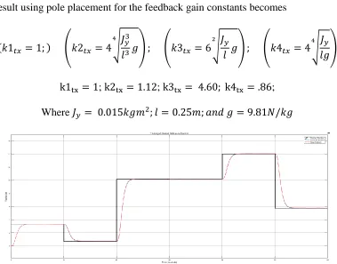
The result using pole placement for the feedback gain constants becomes

(𝑘1𝑡𝑥 = 1; ) (𝑘2𝑡𝑥 = 4 √ 𝐽𝑦3 𝑙3𝑔

4

) ; (𝑘3𝑡𝑥 = 6√ 𝐽𝑦

𝑙 𝑔

2

) ; (𝑘4𝑡𝑥 = 4 √ 𝐽𝑦 𝑙𝑔

4

)

k1_tx = 1; k2_tx = 1.12; k3_tx = 4.60; k4_tx = .86; Where 𝐽𝑦 = 0.015𝑘𝑔𝑚2; 𝑙 = 0.25𝑚; 𝑎𝑛𝑑 𝑔 = 9.81𝑁/𝑘𝑔

Figure 5.14: Roll Position Tracking without Varying Input Uncertainties

(42)

32

of the pitch angle, but to maintain small angle approximation, 𝜃 should not exceed 14𝑜 or 0.244rad. However, when position is greater than 1.4m as shown in figure 5.16, the pitch angle is greater than 0.244rad and if our desired position is as high as 25m, 𝜃 would be higher than 360𝑜 or 3.14rad which makes no sense for the quadrotor to completely rotate and possibly leads to more difficulty for the control of the quad.

Figure 5.15: Pitch Angle at a Desired Position of 1.4m

Figure 5:16 Pitch angle at a desired position of 25m

The problem with limitation is that it could affect state feedback control law and to avoid that, we would have to first limit tracking error. Where

𝑒_𝑡𝑥 = 𝑥_𝑡𝑥+ 𝑒_{𝑡𝑥𝑙𝑖𝑚𝑖𝑡}

𝑒_{𝑡𝑥𝑙𝑖𝑚𝑖𝑡} = −3𝑚 < 𝑒_𝑡𝑥 < 3𝑚

(43)

33

From equation 5.60, if the error between the reference input and the actual position is greater than 3m, then 𝑒_{𝑡𝑥𝑙𝑖𝑚𝑖𝑡} is equal to 3m and if less than -3m then 𝑒_{𝑡𝑥𝑙𝑖𝑚𝑖𝑡} is equal to -3m. By using this technique, the tracking error cannot exceed 3m even if the actual reference is greater than 3m. With the limitation in place, it takes a longer time for the quadrotor to reach desired position. Also 3m was the best limitation that would result in a faster response and still maintain small angle approximation at a degree higher than

14𝑜. Figure 5.17 and figure 5.18 shows the pitch angle remains same even if the distance is greater than 1.4m. Figure 5.19 and 5.20 shows the response of the quadrotor at 1.4m and at 25m.

Figure 5.17: Pitch Angle with Desired Position of 25m

(44)

34

Figure 5.19: Tracking of Desired Position of 1.4m with Pitch Angle Limitation

Figure 5.20: Tracking of Desired Position of 25m with Pitch Angle Limitation Unlike the altitude controller we cannot directly affect translation without affecting rotation. Therefore, we have matched and unmatched uncertainty. Figure 5.21 provides a simulation where unmatched uncertainties were not compensated for and in other to compensate for these uncertainties, the model of the system is redefined as

𝑥̇(𝑡) = 𝐴_𝑚𝑥(𝑡) + 𝐵_𝑚((𝑢(𝑡) + 𝜎_𝑚(𝑡)) + 𝐵𝑢𝑚𝜎𝑢𝑚 (5.61)

Where

𝐵𝑢𝑚 ∈ ℝ𝑛×𝑛(−𝑚) Is a matrix such that 𝐵𝑢𝑚𝑇 = 0 and rank([𝐵𝑚𝐵𝑢𝑚]) = 𝑛

There for

𝐵𝑚=

[ 0 0 0 𝑙

𝐽𝑦]

𝑈𝑡𝑥 𝑎𝑛𝑑 𝐵𝑢𝑚= [

0 𝑔 0 0

(45)

35

The control law for the controller to compensate for unmatched uncertainty would be defined as

𝑈 = −𝐶1(𝑆)𝜎̂𝑚− 𝐶2𝐻𝑚−1𝐻𝑢𝑚𝜎̂𝑢𝑚+ 𝐾𝑔𝑟 (5.63)

Where

𝐶1& 𝐶2 are the low pass filter; 𝐻𝑚 = 𝐶[𝑠𝐼 − 𝐴𝑚]−1𝐵𝑚 and 𝐻𝑢𝑚 = 𝐶[𝑠𝐼 − 𝐴𝑚]−1𝐵𝑢𝑚.

𝐶₂𝐻_𝑚−1_𝐻

𝑢𝑚𝜎̂𝑢𝑚 is needed to cancel the effect of unmatched uncertainty. In this paper, 𝐶2

filter would be a third order low pass filter. It is needed because it makes the transfer function of 𝐶₂𝐻_𝑚−1_𝐻

𝑢𝑚𝜎̂𝑢𝑚 a proper transfer function. At a filter bandwidth of 100,

𝐶2𝐻𝑚−1Hum=

60s2+ 860s + 4600

s3_{+ 24.14s}2_{+ 241.4s + 1000} (5.64)

P matrix to satisfy Lyapunov equation

P = [

1.36 0.50 0.21 0.05 0.50 2.08 0.05 2.20 0.21 0.05 2.22 0.50 0.05 2.20 0.50 5.51

] (5.65)

θ̂̇m = ΓProj(σ̂(t), − (0.834x̃ + 36.674x̃̇ + 8.335θ̃ + 91.852θ̃̇)) (5.66)

θ̂̇_um = ΓProj(σ̂(t), − (4.905x̃ + 20.405x̃̇ + 0.491θ̃ + 21.582θ̃̇)) (5.67)

The adaptation law for matched uncertainties does not include does not include movement on the translational axis and therefore adaptation law for unmatched uncertainties does not include movement on the rotational axis and can be shown in the equation below.

θ̂̇𝑚 = ΓProj(𝜎̂(𝑡), − (0𝑥̃ + 0𝑥̃̇ + 8.335𝜃̃ + 91.852𝜃̃̇)) (5.68)

θ̂̇_𝑢𝑚 = ΓProj(𝜎̂(𝑡), − (4.905𝑥̃ + 20.405𝑥̃̇ + 0𝜃̃ + 0𝜃̃̇)) (5.69)

𝐺_{ℒ1,𝑡𝑥(𝑚𝑎𝑡𝑐ℎ𝑒𝑑)}= [[𝑠𝐼 − 𝐴_𝑚]−1_𝐵

(46)

36

=

[

1.635𝑒06𝑠3_{+ 3.925𝑒08𝑠}2_{+ 3.925𝑒10𝑠}

10000𝑠7_{+ 2.543𝑒06𝑠}6_{+ 2.752𝑒08𝑠}5_{+ 1.363𝑒10𝑠}4_{+ 1.621𝑒11𝑠}3_{+ 8.11𝑒11𝑠}2_{+ 1.871𝑒12𝑠 + 1.635𝑒12}

1.635𝑒06𝑠4_{+ 3.925𝑒08𝑠}3_{+ 3.925𝑒10𝑠}2

10000𝑠7_{+ 2.543𝑒06𝑠}6_{+ 2.752𝑒08𝑠}5_{+ 1.363𝑒10𝑠}4_{+ 1.621𝑒11𝑠}3_{+ 8.11𝑒11𝑠}2_{+ 1.871𝑒12𝑠 + 1.635𝑒12}

1.635𝑒06𝑠5_{+ 3.925𝑒08𝑠}4_{+ 3.925𝑒10𝑠}3

10000𝑠7_{+ 2.543𝑒06𝑠}6_{+ 2.752𝑒08𝑠}5_{+ 1.363𝑒10𝑠}4_{+ 1.621𝑒11𝑠}3_{+ 8.11𝑒11𝑠}2_{+ 1.871𝑒12𝑠 + 1.635𝑒12}

1.635𝑒06𝑠6_{+ 3.925𝑒08𝑠}5_{+ 3.925𝑒10𝑠}4

10000𝑠7_{+ 2.543𝑒06𝑠}6_{+ 2.752𝑒08𝑠}5_{+ 1.363𝑒10𝑠}4_{+ 1.621𝑒11𝑠}3_{+ 8.11𝑒11𝑠}2_{+ 1.871𝑒12𝑠 + 1.635𝑒12]}

(5.71)

𝐺ℒ1,𝑡𝑥(𝑢𝑛𝑚𝑎𝑡𝑐ℎ𝑒𝑑)= [[𝑠𝐼 − 𝐴𝑚]−1𝐵𝑢𝑚][1 − 𝐶𝑟,𝑧(𝑠)] (5.72)

=

[

1.635𝑒06 𝑠^5 + 3.939𝑒08 𝑠^4 + 3.959𝑒10 𝑠^3 + 3.554𝑒10 𝑠^2 + 1.805𝑒11 𝑠

10000𝑠7_{+ 2.543𝑒06𝑠}6_{+ 2.752𝑒08𝑠}5_{+ 1.363𝑒10𝑠}4_{+ 1.621𝑒11𝑠}3_{+ 8.11𝑒11𝑠}2_{+ 1.871𝑒12𝑠 + 1.635𝑒12}

1.635𝑒06 𝑠^6 + 3.939𝑒08 𝑠^5 + 3.959𝑒10 𝑠^4 + 3.554𝑒10 𝑠^3 + 1.805𝑒11 𝑠^2

10000𝑠7_{+ 2.543𝑒06𝑠}6_{+ 2.752𝑒08𝑠}5_{+ 1.363𝑒10𝑠}4_{+ 1.621𝑒11𝑠}3_{+ 8.11𝑒11𝑠}2_{+ 1.871𝑒12𝑠 + 1.635𝑒12}

−1.832𝑒06 𝑠^4 − 4.412𝑒08 𝑠^3 − 4.435𝑒10 𝑠^2 − 3.925𝑒10 𝑠

10000𝑠7_{+ 2.543𝑒06𝑠}6_{+ 2.752𝑒08𝑠}5_{+ 1.363𝑒10𝑠}4_{+ 1.621𝑒11𝑠}3_{+ 8.11𝑒11𝑠}2_{+ 1.871𝑒12𝑠 + 1.635𝑒12}

−1.832𝑒06 𝑠^5 − 4.412𝑒08 𝑠^4 − 4.435𝑒10 𝑠^3 − 3.925𝑒10 𝑠^2

10000𝑠7_{+ 2.543𝑒06𝑠}6_{+ 2.752𝑒08𝑠}5_{+ 1.363𝑒10𝑠}4_{+ 1.621𝑒11𝑠}3_{+ 8.11𝑒11𝑠}2_{+ 1.871𝑒12𝑠 + 1.635𝑒12]}

(5.73)

‖𝐺ℒ1,𝑡𝑥(𝑚𝑎𝑡𝑐ℎ𝑒𝑑)‖_ℒ1 = 0.008which give us an uncertainty limit of 125N. With that, the

adaptation gain can be big enough for faster adaptation. From equation 5.68, 𝜃̃ = 𝜃̂ − 𝜃

and 𝜃̃̇ = 𝜃̂̇ − 𝜃̇. For simulation, a varying uncertainty of -10N to 10N would be used with an adaptation gain of 10000.

‖𝐺_{ℒ1,𝑡𝑥(𝑢𝑛𝑚𝑎𝑡𝑐ℎ𝑒𝑑)}‖

ℒ1 = 0.056which give us an uncertainty limit of 17.54N. From

equation 5.69, 𝑥̃ = 𝑥̂ − 𝑥 and 𝑥̃̇ = 𝑥̇ − 𝑥. For simulation, a varying uncertainty of -10N to 10N would be used with an adaptation gain of 10000.

(47)

37

Figure 5.22: Roll Position Tracking with Varying Matched Uncertainties

Figure 5.23: Structural Design for Roll Controller

(48)

38

Figure 5.25: Estimate Uncertainty vs Real Uncertainty for Unmatched Uncertainties Roll Control

Figure 5.26: Roll Position Tracking with Varying Matched and Unmatched Uncertainties

5.7 TRANSLATION CONTROL ALONG THE Y AXIS

This controller design is similar for the controller design for translation about the x axis, so controller output for movement is

𝑢𝑡𝑦 = (𝑒𝑡𝑦− 𝑘1𝑡𝑥x − 𝑘2𝑡𝑥𝑥̇ − 𝑘3𝑡𝑥(𝜙) − 𝑘4𝑡𝑥(𝜙̇))

You notice there is no multiplication of (-1) at the dynamic model which is the only difference between both design. Therefore

(49)

39

Figure 5.27: Feedback Response without Disturbance

Figure 5.28: Pitch Position Tracking with Varying Matched and Unmatched [Y-Axis]

(50)

40

(51)

41

CHAPTER 6 CONTROLLER SIMULATION WITH NON-LINEAR MODEL

In Chapter 5, controllers were designed based on a linearized model of the quadrotor, but in this chapter 6, the nonlinear model is used. The non-linear model is based on what was discussed in chapter 3 and in addition to the model we would calculate the thrust generated by each motor as shown below. These thrusts are mathematical relations that were discussed in chapter 3 from equation 3.6-3.9.

[ 𝐹1 𝐹₂ 𝐹3 𝐹₄ ] = [

1 1 1 1

0 − 1 0 1

1 0 − 1 0

1 − 1 1 − 1 ] −1 [ 𝑈_𝑡𝑧 𝑈_𝑡𝑥 𝑈_𝑡𝑦 𝑈_𝑟𝑧 ]

For the simulation, the table below shows the disturbances that were used on the quadrotor model.

Tz Disturbance -10< 𝑇𝑧 < 10

Ty Disturbance -0.4< 𝑇𝑦 < 0.4

Tx Disturbance -0.4< 𝑇𝑥 < 0.4

Rz disturbance -10< 𝑇𝑧 < 10

Ry disturbance -12< 𝑅𝑦 < 12

Rx disturbance -12< 𝑅𝑥 < 12

Tz Extra mass -5< 𝑇𝑧 < 5

(52)

42

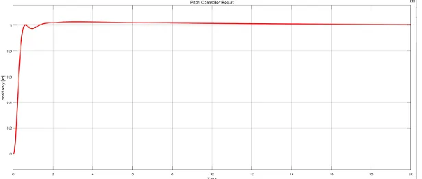
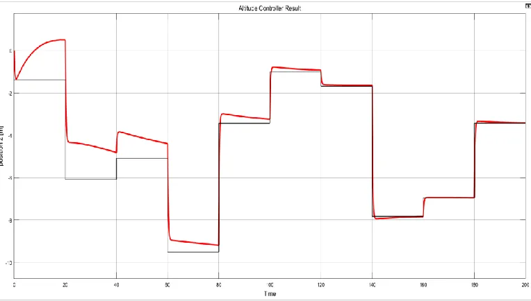
Figure 6.1-6.4 shows the quadrotor response to desired position or location. It is exactly same as most of the result shown in chapter 5. To avoid repetition of results such as tracking of uncertainties, pitch and roll limitation would be avoided. Figure 6.5 and 6.6 provides the overall Simulink design and each detail in each subsystem have been discussed from chapter 3 to chapter 5.

Figure 6.2: Altitude Position Tracking Using ℒ₁ Adaptive Controller [Z-Axis]

Figure 6.3: Yaw Position Yaw Position Tracking Using ℒ₁ Adaptive Controller [Z-Axis]

(53)

43

Figure 6.5: Pitch Position Tracking Using ℒ₁ Adaptive Controller [Y-Axis]

(54)

44

(55)

45

CHAPTER 7 SUMMARY AND CONCLUSION

The main goal of this thesis is to design a controller that can control a quadrotor in the presence of disturbance or uncertainties. Although they are different control method used such as PID controller, this paper focused on the application of ℒ₁ adaptive controller in simulation. This paper includes the linear and non-linear dynamic model of the quadrotor, application using PID controller, ℒ1 adaptive controller, and resistance to

uncertainties. As figure 4.10 shows, when a step disturbance is added to the input of the altitude controller, it took about 160 seconds for the quadrotor to adapt so the main advantage of ℒ1 adaptive controller over PID controller is its fast adaptation to

uncertainties or disturbance because of its high adaptation gain.

In the process of designing ℒ₁ adaptive controller for the quadrotor, various limitations and problems are taking into consideration such as the under actuation of the quadrotor, presentation of matched and unmatched uncertainties, addition of extra mass and failure of rotating motor. All these limitations were taking care of in this paper, except for failure of the rotating motor. Theoretically when there is a motor failure, it is difficult to have a stable flight. To avoid these problems, a different technique would be used for future work. Future work would also focus on the implementation of ℒ1 adaptive controller

(56)

46

(57)

47

REFERENCES

Bouabdallah, Samir and Siegwart, Roland. 2007. Full Control of Quadrotor. Autonomous Systems Lab: Swiss Federal Institute of Technology, ETHZ Zurich, Switzerland. Brudigam, Tim. 2014. Fault-Tolerant Control of Quadrotor. Thesis, Technical University

of Munich.

ElKholy, Heba talla Mohamed Nabil. 2014. Dynamic Modeling and Control of a Quadrotor Using Linear and Nonlinear Approaches. Thesis, America University in Cairo.

Hovakimyan, Naira. 2013. ℒ1 Adaptive Control and Its Transition to Practice. Department

of Mechanical Science and Engineering University of Illinois.

Hovakimyan, Naira. 2013. ℒ1 Adaptive Control. Department of Mechanical Science and

Engineering University of Illinois.

Hovakimyan, Naira and Cao, Chengyu. 2010. ℒ₁ Adaptive Control Theory: Guaranteed Robustness with Fast Adaptation. Philadelphia: Society for Industrial & Applied Mathematics, U.S.

Murray, M. Richard and Aström, J. Karl. 2009. Feedback Systems: An introduction for Scientist and Engineering. Princeton: Princeton University Press.

Premerlani, William and Bizard, Paul. 2009. Direction Cosine Matrix IMU: Theory.

Retrieved from Web.

(58)

48

Schmidt, M. David. 2011. Simulation and Control of a Quadrotor Unmanned Aerial Vehicle. University of Kentucky Library.

Seiler, Peter, Dorobantu, Andrei and Balas, Gary. 2010. Robustness Analysis of an

ℒ₁Adaptive Controller. AIAA Guidance, Navigation, and Control Conference. Wang, Xiaofeng and Hovakimyan, Naira. 2012. ℒ₁ Adaptive Controller for Nonlinear